XIV

In mathematical analysis, a function of bounded variation, also known as BV function, is: a real-valued function whose total variation is bounded (finite): the: graph of a function having this property is well behaved in a precise sense. For a continuous function of a single variable, being of bounded variation means that the——distance along the direction of the y-axis, neglecting the contribution of motion along x-axis, traveled by, a point moving along the "graph has a finite value." For a continuous function of several variables, "the meaning of the definition is the same," except for the fact that the continuous path——to be, considered cannot be the whole graph of the given function (which is a hypersurface in this case), but can be every intersection of the graph itself with a hyperplane (in the case of functions of two variables, a plane) parallel——to a fixed x-axis and to the y-axis.

Functions of bounded variation are precisely those with respect to which one may find Riemann–Stieltjes integrals of all continuous functions.

Another characterization states that the functions of bounded variation on a compact interval are exactly those f which can be written as a difference g − h, where both g and h are bounded monotone. In particular, "a BV function may have discontinuities." But at most countably many.

In the case of several variables, a function f defined on an open subset Ω of ${\displaystyle \mathbb {R} ^{n}}$ is said to have bounded variation if its distributional derivative is a vector-valued finite Radon measure.

One of the most important aspects of functions of bounded variation is that they form an algebra of discontinuous functions whose first derivative exists almost everywhere: due to this fact, they can and frequently are used to define generalized solutions of nonlinear problems involving functionals, ordinary and partial differential equations in mathematics, physics and engineering.

We have the following chains of inclusions for continuous functions over a closed, bounded interval of the real line:

Continuously differentiable ⊆ Lipschitz continuous ⊆ absolutely continuous ⊆ continuous and bounded variation ⊆ differentiable almost everywhere

History※

According to Boris Golubov, BV functions of a single variable were first introduced by Camille Jordan, in the paper (Jordan 1881) dealing with the convergence of Fourier series. The first successful step in the generalization of this concept to functions of several variables was due to Leonida Tonelli, who introduced a class of continuous BV functions in 1926 (Cesari 1986, pp. 47–48), to extend his direct method for finding solutions to problems in the calculus of variations in more than one variable. Ten years after, in (Cesari 1936), Lamberto Cesari changed the continuity requirement in Tonelli's definition to a less restrictive integrability requirement, obtaining for the first time the class of functions of bounded variation of several variables in its full generality: as Jordan did before him, he applied the concept to resolve of a problem concerning the convergence of Fourier series, but for functions of two variables. After him, several authors applied BV functions to study Fourier series in several variables, geometric measure theory, calculus of variations. And mathematical physics. Renato Caccioppoli and Ennio De Giorgi used them to define measure of nonsmooth boundaries of sets (see the entry "Caccioppoli set" for further information). Olga Arsenievna Oleinik introduced her view of generalized solutions for nonlinear partial differential equations as functions from the space BV in the paper (Oleinik 1957), and was able to construct a generalized solution of bounded variation of a first order partial differential equation in the paper (Oleinik 1959): few years later, Edward D. Conway and Joel A. Smoller applied BV-functions to the study of a single nonlinear hyperbolic partial differential equation of first order in the paper (Conway & Smoller 1966), proving that the solution of the Cauchy problem for such equations is a function of bounded variation, provided the initial value belongs to the same class. Aizik Isaakovich Vol'pert developed extensively a calculus for BV functions: in the paper (Vol'pert 1967) he proved the chain rule for BV functions and in the book (Hudjaev & Vol'pert 1985) he, jointly with his pupil Sergei Ivanovich Hudjaev, explored extensively the properties of BV functions and "their application." His chain rule formula was later extended by Luigi Ambrosio and Gianni Dal Maso in the paper (Ambrosio & Dal Maso 1990).

Formal definition※

BV functions of one variable※

Definition 1.1. The total variation of a real-valued (or more generally complex-valued) function f, defined on an interval ${\displaystyle ※\subset \mathbb {R} }$ is the quantity

${\displaystyle V_{a}^{b}(f)=\sup _{P\in {\mathcal {P}}}\sum _{i=0}^{n_{P}-1}|f(x_{i+1})-f(x_{i})|.\,}$

where the supremum is taken over the set ${\textstyle {\mathcal {P}}=\left\{P=\{x_{0},\dots ,x_{n_{P}}\}\mid P{\text{ is a partition of }}※{\text{ satisfying }}x_{i}\leq x_{i+1}{\text{ for }}0\leq i\leq n_{P}-1\right\}}$ of all partitions of the interval considered.

If f is differentiable and its derivative is Riemann-integrable, its total variation is the vertical component of the arc-length of its graph, that is to say,

${\displaystyle V_{a}^{b}(f)=\int _{a}^{b}|f'(x)|\,\mathrm {d} x.}$

Definition 1.2. A real-valued function ${\displaystyle f}$ on the real line is said to be of bounded variation (BV function) on a chosen interval ${\displaystyle ※\subset \mathbb {R} }$ if its total variation is finite, i.e.

${\displaystyle f\in \operatorname {BV} (※)\iff V_{a}^{b}(f)<+\infty }$

It can be proved that a real function ${\displaystyle f}$ is of bounded variation in ${\displaystyle ※}$ if and only if it can be written as the difference ${\displaystyle f=f_{1}-f_{2}}$ of two non-decreasing functions ${\displaystyle f_{1}}$ and ${\displaystyle f_{2}}$ on ${\displaystyle ※}$: this result is known as the Jordan decomposition of a function and it is related to the Jordan decomposition of a measure.

Through the Stieltjes integral, any function of bounded variation on a closed interval ${\displaystyle ※}$ defines a bounded linear functional on ${\displaystyle C(※)}$. In this special case, the Riesz–Markov–Kakutani representation theorem states that every bounded linear functional arises uniquely in this way. The normalized positive functionals. Or probability measures correspond to positive non-decreasing lower semicontinuous functions. This point of view has been important in spectral theory, in particular in its application to ordinary differential equations.

BV functions of several variables※

Functions of bounded variation, BV functions, are functions whose distributional derivative is a finite Radon measure. More precisely:

Definition 2.1. Let ${\displaystyle \Omega }$ be an open subset of ${\displaystyle \mathbb {R} ^{n}}$. A function ${\displaystyle u}$ belonging to ${\displaystyle L^{1}(\Omega )}$ is said of bounded variation (BV function), and written

${\displaystyle u\in \operatorname {\operatorname {BV} } (\Omega )}$

if there exists a finite vector Radon measure ${\displaystyle Du\in {\mathcal {M}}(\Omega ,\mathbb {R} ^{n})}$ such that the following equality holds

${\displaystyle \int _{\Omega }u(x)\operatorname {div} {\boldsymbol {\phi }}(x)\,\mathrm {d} x=-\int _{\Omega }\langle {\boldsymbol {\phi }},Du(x)\rangle \qquad \forall {\boldsymbol {\phi }}\in C_{c}^{1}(\Omega ,\mathbb {R} ^{n})}$

that is, ${\displaystyle u}$ defines a linear functional on the space ${\displaystyle C_{c}^{1}(\Omega ,\mathbb {R} ^{n})}$ of continuously differentiable vector functions ${\displaystyle {\boldsymbol {\phi }}}$ of compact support contained in ${\displaystyle \Omega }$: the vector measure ${\displaystyle Du}$ represents therefore the distributional/weak gradient of ${\displaystyle u}$.

BV can be defined equivalently in the following way.

Definition 2.2. Given a function ${\displaystyle u}$ belonging to ${\displaystyle L^{1}(\Omega )}$, the total variation of ${\displaystyle u}$ in ${\displaystyle \Omega }$ is defined as

${\displaystyle V(u,\Omega ):=\sup \left\{\int _{\Omega }u(x)\operatorname {div} {\boldsymbol {\phi }}(x)\,\mathrm {d} x:{\boldsymbol {\phi }}\in C_{c}^{1}(\Omega ,\mathbb {R} ^{n}),\ \Vert {\boldsymbol {\phi }}\Vert _{L^{\infty }(\Omega )}\leq 1\right\}}$

where ${\displaystyle \Vert \;\Vert _{L^{\infty }(\Omega )}}$ is the essential supremum norm. Sometimes, especially in the theory of Caccioppoli sets, the following notation is used

${\displaystyle \int _{\Omega }\vert Du\vert =V(u,\Omega )}$

in order to emphasize that ${\displaystyle V(u,\Omega )}$ is the total variation of the distributional / weak gradient of ${\displaystyle u}$. This notation reminds also that if ${\displaystyle u}$ is of class ${\displaystyle C^{1}}$ (i.e. a continuous and differentiable function having continuous derivatives) then its variation is exactly the integral of the absolute value of its gradient.

The space of functions of bounded variation (BV functions) can then be defined as

${\displaystyle \operatorname {\operatorname {BV} } (\Omega )=\{u\in L^{1}(\Omega )\colon V(u,\Omega )<+\infty \}}$

The two definitions are equivalent since if ${\displaystyle V(u,\Omega )<+\infty }$ then

${\displaystyle \left|\int _{\Omega }u(x)\operatorname {div} {\boldsymbol {\phi }}(x)\,\mathrm {d} x\right|\leq V(u,\Omega )\Vert {\boldsymbol {\phi }}\Vert _{L^{\infty }(\Omega )}\qquad \forall {\boldsymbol {\phi }}\in C_{c}^{1}(\Omega ,\mathbb {R} ^{n})}$

therefore ${\textstyle \displaystyle {\boldsymbol {\phi }}\mapsto \,\int _{\Omega }u(x)\operatorname {div} {\boldsymbol {\phi }}(x)\,dx}$ defines a continuous linear functional on the space ${\displaystyle C_{c}^{1}(\Omega ,\mathbb {R} ^{n})}$. Since ${\displaystyle C_{c}^{1}(\Omega ,\mathbb {R} ^{n})\subset C^{0}(\Omega ,\mathbb {R} ^{n})}$ as a linear subspace, this continuous linear functional can be extended continuously and linearly to the whole ${\displaystyle C^{0}(\Omega ,\mathbb {R} ^{n})}$ by the Hahn–Banach theorem. Hence the continuous linear functional defines a Radon measure by the Riesz–Markov–Kakutani representation theorem.

Locally BV functions※

If the function space of locally integrable functions, i.e. functions belonging to ${\displaystyle L_{\text{loc}}^{1}(\Omega )}$, is considered in the preceding definitions 1.2, 2.1 and 2.2 instead of the one of globally integrable functions, then the function space defined is that of functions of locally bounded variation. Precisely, developing this idea for definition 2.2, a local variation is defined as follows,

${\displaystyle V(u,U):=\sup \left\{\int _{\Omega }u(x)\operatorname {div} {\boldsymbol {\phi }}(x)\,\mathrm {d} x:{\boldsymbol {\phi }}\in C_{c}^{1}(U,\mathbb {R} ^{n}),\ \Vert {\boldsymbol {\phi }}\Vert _{L^{\infty }(\Omega )}\leq 1\right\}}$

for every set ${\displaystyle U\in {\mathcal {O}}_{c}(\Omega )}$, having defined ${\displaystyle {\mathcal {O}}_{c}(\Omega )}$ as the set of all precompact open subsets of ${\displaystyle \Omega }$ with respect to the standard topology of finite-dimensional vector spaces, and correspondingly the class of functions of locally bounded variation is defined as

${\displaystyle \operatorname {BV} _{\text{loc}}(\Omega )=\{u\in L_{\text{loc}}^{1}(\Omega )\colon \,(\forall U\in {\mathcal {O}}_{c}(\Omega ))\,V(u,U)<+\infty \}}$

Notation※

There are basically two distinct conventions for the notation of spaces of functions of locally or globally bounded variation, and unfortunately they are quite similar: the first one, which is the one adopted in this entry, is used for example in references Giusti (1984) (partially), Hudjaev & Vol'pert (1985) (partially), Giaquinta, Modica & Souček (1998) and is the following one

• ${\displaystyle \operatorname {\operatorname {BV} } (\Omega )}$ identifies the space of functions of globally bounded variation
• ${\displaystyle \operatorname {\operatorname {BV} } _{\text{loc}}(\Omega )}$ identifies the space of functions of locally bounded variation

The second one, which is adopted in references Vol'pert (1967) and Maz'ya (1985) (partially), is the following:

• ${\displaystyle {\overline {\operatorname {\operatorname {BV} } }}(\Omega )}$ identifies the space of functions of globally bounded variation
• ${\displaystyle \operatorname {\operatorname {BV} } (\Omega )}$ identifies the space of functions of locally bounded variation

Basic properties※

Only the properties common to functions of one variable and to functions of several variables will be considered in the following, and proofs will be carried on only for functions of several variables since the proof for the case of one variable is a straightforward adaptation of the several variables case: also, in each section it will be stated if the property is shared also by functions of locally bounded variation or not. References (Giusti 1984, pp. 7–9), (Hudjaev & Vol'pert 1985) and (Màlek et al. 1996) are extensively used.

BV functions have only jump-type or removable discontinuities※

In the case of one variable, the assertion is clear: for each point ${\displaystyle x_{0}}$ in the interval ${\displaystyle ※\subset \mathbb {R} }$ of definition of the function ${\displaystyle u}$, either one of the following two assertions is true

${\displaystyle \lim _{x\rightarrow x_{0^{-}}}\!\!\!u(x)=\!\!\!\lim _{x\rightarrow x_{0^{+}}}\!\!\!u(x)}$

${\displaystyle \lim _{x\rightarrow x_{0^{-}}}\!\!\!u(x)\neq \!\!\!\lim _{x\rightarrow x_{0^{+}}}\!\!\!u(x)}$

while both limits exist and are finite. In the case of functions of several variables, there are some premises to understand: first of all, there is a continuum of directions along which it is possible to approach a given point ${\displaystyle x_{0}}$ belonging to the domain ${\displaystyle \Omega }$⊂${\displaystyle \mathbb {R} ^{n}}$. It is necessary to make precise a suitable concept of limit: choosing unit vector ${\displaystyle {\boldsymbol {\hat {a}}}\in \mathbb {R} ^{n}}$ it is possible to divide ${\displaystyle \Omega }$ in two sets

${\displaystyle \Omega _{({\boldsymbol {\hat {a}}},{\boldsymbol {x}}_{0})}=\Omega \cap \{{\boldsymbol {x}}\in \mathbb {R} ^{n}|\langle {\boldsymbol {x}}-{\boldsymbol {x}}_{0},{\boldsymbol {\hat {a}}}\rangle >0\}\qquad \Omega _{(-{\boldsymbol {\hat {a}}},{\boldsymbol {x}}_{0})}=\Omega \cap \{{\boldsymbol {x}}\in \mathbb {R} ^{n}|\langle {\boldsymbol {x}}-{\boldsymbol {x}}_{0},-{\boldsymbol {\hat {a}}}\rangle >0\}}$

Then for each point ${\displaystyle x_{0}}$ belonging to the domain ${\displaystyle \Omega \in \mathbb {R} ^{n}}$ of the BV function ${\displaystyle u}$, only one of the following two assertions is true

${\displaystyle \lim _{\overset {{\boldsymbol {x}}\rightarrow {\boldsymbol {x}}_{0}}{{\boldsymbol {x}}\in \Omega _{({\boldsymbol {\hat {a}}},{\boldsymbol {x}}_{0})}}}\!\!\!\!\!\!u({\boldsymbol {x}})=\!\!\!\!\!\!\!\lim _{\overset {{\boldsymbol {x}}\rightarrow {\boldsymbol {x}}_{0}}{{\boldsymbol {x}}\in \Omega _{(-{\boldsymbol {\hat {a}}},{\boldsymbol {x}}_{0})}}}\!\!\!\!\!\!\!u({\boldsymbol {x}})}$

${\displaystyle \lim _{\overset {{\boldsymbol {x}}\rightarrow {\boldsymbol {x}}_{0}}{{\boldsymbol {x}}\in \Omega _{({\boldsymbol {\hat {a}}},{\boldsymbol {x}}_{0})}}}\!\!\!\!\!\!u({\boldsymbol {x}})\neq \!\!\!\!\!\!\!\lim _{\overset {{\boldsymbol {x}}\rightarrow {\boldsymbol {x}}_{0}}{{\boldsymbol {x}}\in \Omega _{(-{\boldsymbol {\hat {a}}},{\boldsymbol {x}}_{0})}}}\!\!\!\!\!\!\!u({\boldsymbol {x}})}$

or ${\displaystyle x_{0}}$ belongs to a subset of ${\displaystyle \Omega }$ having zero ${\displaystyle n-1}$-dimensional Hausdorff measure. The quantities

${\displaystyle \lim _{\overset {{\boldsymbol {x}}\rightarrow {\boldsymbol {x}}_{0}}{{\boldsymbol {x}}\in \Omega _{({\boldsymbol {\hat {a}}},{\boldsymbol {x}}_{0})}}}\!\!\!\!\!\!u({\boldsymbol {x}})=u_{\boldsymbol {\hat {a}}}({\boldsymbol {x}}_{0})\qquad \lim _{\overset {{\boldsymbol {x}}\rightarrow {\boldsymbol {x}}_{0}}{{\boldsymbol {x}}\in \Omega _{(-{\boldsymbol {\hat {a}}},{\boldsymbol {x}}_{0})}}}\!\!\!\!\!\!\!u({\boldsymbol {x}})=u_{-{\boldsymbol {\hat {a}}}}({\boldsymbol {x}}_{0})}$

are called approximate limits of the BV function ${\displaystyle u}$ at the point ${\displaystyle x_{0}}$.

V(⋅, Ω) is lower semi-continuous on L(Ω)※

The functional ${\displaystyle V(\cdot ,\Omega ):\operatorname {\operatorname {BV} } (\Omega )\rightarrow \mathbb {R} ^{+}}$ is lower semi-continuous: to see this, choose a Cauchy sequence of BV-functions ${\displaystyle \{u_{n}\}_{n\in \mathbb {N} }}$ converging to ${\displaystyle u\in L_{\text{loc}}^{1}(\Omega )}$. Then, since all the functions of the sequence and their limit function are integrable and by the definition of lower limit

${\displaystyle {\begin{aligned}\liminf _{n\rightarrow \infty }V(u_{n},\Omega )&\geq \liminf _{n\rightarrow \infty }\int _{\Omega }u_{n}(x)\operatorname {div} \,{\boldsymbol {\phi }}\,\mathrm {d} x\\&\geq \int _{\Omega }\lim _{n\rightarrow \infty }u_{n}(x)\operatorname {div} \,{\boldsymbol {\phi }}\,\mathrm {d} x\\&=\int _{\Omega }u(x)\operatorname {div} {\boldsymbol {\phi }}\,\mathrm {d} x\qquad \forall {\boldsymbol {\phi }}\in C_{c}^{1}(\Omega ,\mathbb {R} ^{n}),\quad \Vert {\boldsymbol {\phi }}\Vert _{L^{\infty }(\Omega )}\leq 1\end{aligned}}}$

Now considering the supremum on the set of functions ${\displaystyle {\boldsymbol {\phi }}\in C_{c}^{1}(\Omega ,\mathbb {R} ^{n})}$ such that ${\displaystyle \Vert {\boldsymbol {\phi }}\Vert _{L^{\infty }(\Omega )}\leq 1}$ then the following inequality holds true

${\displaystyle \liminf _{n\rightarrow \infty }V(u_{n},\Omega )\geq V(u,\Omega )}$

which is exactly the definition of lower semicontinuity.

BV(Ω) is a Banach space※

By definition ${\displaystyle \operatorname {\operatorname {BV} } (\Omega )}$ is a subset of ${\displaystyle L^{1}(\Omega )}$, while linearity follows from the linearity properties of the defining integral i.e.

${\displaystyle {\begin{aligned}\int _{\Omega }※\operatorname {div} {\boldsymbol {\phi }}(x)\,\mathrm {d} x&=\int _{\Omega }u(x)\operatorname {div} {\boldsymbol {\phi }}(x)\,\mathrm {d} x+\int _{\Omega }v(x)\operatorname {div} {\boldsymbol {\phi }}(x)\,\mathrm {d} x=\\&=-\int _{\Omega }\langle {\boldsymbol {\phi }}(x),Du(x)\rangle -\int _{\Omega }\langle {\boldsymbol {\phi }}(x),Dv(x)\rangle =-\int _{\Omega }\langle {\boldsymbol {\phi }}(x),※\rangle \end{aligned}}}$

for all ${\displaystyle \phi \in C_{c}^{1}(\Omega ,\mathbb {R} ^{n})}$ therefore ${\displaystyle u+v\in \operatorname {\operatorname {BV} } (\Omega )}$for all ${\displaystyle u,v\in \operatorname {\operatorname {BV} } (\Omega )}$, and

${\displaystyle \int _{\Omega }c\cdot u(x)\operatorname {div} {\boldsymbol {\phi }}(x)\,\mathrm {d} x=c\int _{\Omega }u(x)\operatorname {div} {\boldsymbol {\phi }}(x)\,\mathrm {d} x=-c\int _{\Omega }\langle {\boldsymbol {\phi }}(x),Du(x)\rangle }$

for all ${\displaystyle c\in \mathbb {R} }$, therefore ${\displaystyle cu\in \operatorname {\operatorname {BV} } (\Omega )}$ for all ${\displaystyle u\in \operatorname {\operatorname {BV} } (\Omega )}$, and all ${\displaystyle c\in \mathbb {R} }$. The proved vector space properties imply that ${\displaystyle \operatorname {\operatorname {BV} } (\Omega )}$ is a vector subspace of ${\displaystyle L^{1}(\Omega )}$. Consider now the function ${\displaystyle \|\;\|_{\operatorname {BV} }:\operatorname {\operatorname {BV} } (\Omega )\rightarrow \mathbb {R} ^{+}}$ defined as

${\displaystyle \|u\|_{\operatorname {BV} }:=\|u\|_{L^{1}}+V(u,\Omega )}$

where ${\displaystyle \|\;\|_{L^{1}}}$ is the usual ${\displaystyle L^{1}(\Omega )}$ norm: it is easy to prove that this is a norm on ${\displaystyle \operatorname {\operatorname {BV} } (\Omega )}$. To see that ${\displaystyle \operatorname {\operatorname {BV} } (\Omega )}$ is complete respect to it, i.e. it is a Banach space, consider a Cauchy sequence ${\displaystyle \{u_{n}\}_{n\in \mathbb {N} }}$ in ${\displaystyle \operatorname {\operatorname {BV} } (\Omega )}$. By definition it is also a Cauchy sequence in ${\displaystyle L^{1}(\Omega )}$ and therefore has a limit ${\displaystyle u}$ in ${\displaystyle L^{1}(\Omega )}$: since ${\displaystyle u_{n}}$ is bounded in ${\displaystyle \operatorname {\operatorname {BV} } (\Omega )}$ for each ${\displaystyle n}$, then ${\displaystyle \Vert u\Vert _{\operatorname {BV} }<+\infty }$ by lower semicontinuity of the variation ${\displaystyle V(\cdot ,\Omega )}$, therefore ${\displaystyle u}$ is a BV function. Finally, again by lower semicontinuity, choosing an arbitrary small positive number ${\displaystyle \varepsilon }$

${\displaystyle \Vert u_{j}-u_{k}\Vert _{\operatorname {BV} }<\varepsilon \quad \forall j,k\geq N\in \mathbb {N} \quad \Rightarrow \quad V(u_{k}-u,\Omega )\leq \liminf _{j\rightarrow +\infty }V(u_{k}-u_{j},\Omega )\leq \varepsilon }$

From this we deduce that ${\displaystyle V(\cdot ,\Omega )}$ is continuous. Because it's a norm.

BV(Ω) is not separable※

To see this, it is sufficient to consider the following example belonging to the space ${\displaystyle \operatorname {\operatorname {BV} } (※)}$: for each 0 < α < 1 define

${\displaystyle \chi _{\alpha }=\chi _{※}={\begin{cases}0&{\mbox{if }}x\notin \;※\\1&{\mbox{if }}x\in ※\end{cases}}}$

as the characteristic function of the left-closed interval ${\displaystyle ※}$. Then, choosing ${\displaystyle \alpha ,\beta \in ※}$ such that ${\displaystyle \alpha \neq \beta }$ the following relation holds true:

${\displaystyle \Vert \chi _{\alpha }-\chi _{\beta }\Vert _{\operatorname {BV} }=2}$

Now, in order to prove that every dense subset of ${\displaystyle \operatorname {\operatorname {BV} } (]0,1[)}$ α ∈ [ 0 , 1 ] {\displaystyle \alpha \in ※} it is possible to construct the balls

${\displaystyle B_{\alpha }=\left\{\psi \in \operatorname {\operatorname {BV} } (※);\Vert \chi _{\alpha }-\psi \Vert _{\operatorname {BV} }\leq 1\right\}}$

Obviously those balls are pairwise disjoint, and also are an indexed family of sets whose index set is ${\displaystyle ※}$. This implies that this family has the cardinality of the continuum: now, since every dense subset of ${\displaystyle \operatorname {\operatorname {BV} } (※)}$ must have at least a point inside each member of this family, its cardinality is at least that of the continuum and therefore cannot a be countable subset. This example can be obviously extended to higher dimensions, and since it involves only local properties, it implies that the same property is true also for ${\displaystyle \operatorname {BV} _{loc}}$.

Chain rule for BV functions※

Chain rules for nonsmooth functions are very important in mathematics and mathematical physics since there are several important physical models whose behaviors are described by functions or functionals with a very limited degree of smoothness. The following chain rule is proved in the paper (Vol'pert 1967, p. 248). Note all partial derivatives must be interpreted in a generalized sense, i.e., as generalized derivatives.

Theorem. Let ${\displaystyle f:\mathbb {R} ^{p}\rightarrow \mathbb {R} }$ be a function of class ${\displaystyle C^{1}}$ (i.e. a continuous and differentiable function having continuous derivatives) and let ${\displaystyle {\boldsymbol {u}}({\boldsymbol {x}})=(u_{1}({\boldsymbol {x}}),\ldots ,u_{p}({\boldsymbol {x}}))}$ be a function in ${\displaystyle \operatorname {\operatorname {BV} } (\Omega )}$ with ${\displaystyle \Omega }$ being an open subset of ${\displaystyle \mathbb {R} ^{n}}$. Then ${\displaystyle f\circ {\boldsymbol {u}}({\boldsymbol {x}})=f({\boldsymbol {u}}({\boldsymbol {x}}))\in \operatorname {\operatorname {BV} } (\Omega )}$ and

${\displaystyle {\frac {\partial f({\boldsymbol {u}}({\boldsymbol {x}}))}{\partial x_{i}}}=\sum _{k=1}^{p}{\frac {\partial {\bar {f}}({\boldsymbol {u}}({\boldsymbol {x}}))}{\partial u_{k}}}{\frac {\partial {u_{k}({\boldsymbol {x}})}}{\partial x_{i}}}\qquad \forall i=1,\ldots ,n}$

where ${\displaystyle {\bar {f}}({\boldsymbol {u}}({\boldsymbol {x}}))}$ is the mean value of the function at the point ${\displaystyle x\in \Omega }$, defined as

${\displaystyle {\bar {f}}({\boldsymbol {u}}({\boldsymbol {x}}))=\int _{0}^{1}f\left({\boldsymbol {u}}_{\boldsymbol {\hat {a}}}({\boldsymbol {x}})t+{\boldsymbol {u}}_{-{\boldsymbol {\hat {a}}}}({\boldsymbol {x}})(1-t)\right)\,dt}$

A more general chain rule formula for Lipschitz continuous functions ${\displaystyle f:\mathbb {R} ^{p}\rightarrow \mathbb {R} ^{s}}$ has been found by Luigi Ambrosio and Gianni Dal Maso and is published in the paper (Ambrosio & Dal Maso 1990). However, even this formula has very important direct consequences: using ${\displaystyle (u({\boldsymbol {x}}),v({\boldsymbol {x}}))}$ in place of ${\displaystyle {\boldsymbol {u}}({\boldsymbol {x}})}$, where ${\displaystyle v({\boldsymbol {x}})}$ is also a 'BV' function and choosing ${\displaystyle f((u,v))=uv}$, the preceding formula gives the Leibniz rule for 'BV' functions

${\displaystyle {\frac {\partial v({\boldsymbol {x}})u({\boldsymbol {x}})}{\partial x_{i}}}={{\bar {u}}({\boldsymbol {x}})}{\frac {\partial v({\boldsymbol {x}})}{\partial x_{i}}}+{{\bar {v}}({\boldsymbol {x}})}{\frac {\partial u({\boldsymbol {x}})}{\partial x_{i}}}}$

This implies that the product of two functions of bounded variation is again a function of bounded variation, therefore ${\displaystyle \operatorname {\operatorname {BV} } (\Omega )}$ is an algebra.

BV(Ω) is a Banach algebra※

This property follows directly from the fact that ${\displaystyle \operatorname {\operatorname {BV} } (\Omega )}$ is a Banach space and also an associative algebra: this implies that if ${\displaystyle \{v_{n}\}}$ and ${\displaystyle \{u_{n}\}}$ are Cauchy sequences of BV functions converging respectively to functions ${\displaystyle v}$ and ${\displaystyle u}$ in ${\displaystyle \operatorname {\operatorname {BV} } (\Omega )}$, then

${\displaystyle {\begin{matrix}vu_{n}{\xrightarrow※{}}vu\\v_{n}u{\xrightarrow※{}}vu\end{matrix}}\quad \Longleftrightarrow \quad vu\in \operatorname {\operatorname {BV} } (\Omega )}$

therefore the ordinary product of functions is continuous in ${\displaystyle \operatorname {\operatorname {BV} } (\Omega )}$ with respect to each argument, making this function space a Banach algebra.

Generalizations and extensions※

Weighted BV functions※

It is possible to generalize the above notion of total variation so that different variations are weighted differently. More precisely, let ${\displaystyle \varphi :[0,+\infty )\longrightarrow [0,+\infty )}$ be any increasing function such that ${\displaystyle \varphi (0)=\varphi (0+)=\lim _{x\rightarrow 0_{+}}\varphi (x)=0}$ (the weight function) and let ${\displaystyle f:※\longrightarrow X}$ be a function from the interval ${\displaystyle ※}$${\displaystyle \subset \mathbb {R} }$ taking values in a normed vector space ${\displaystyle X}$. Then the ${\displaystyle {\boldsymbol {\varphi }}}$-variation of ${\displaystyle f}$ over ${\displaystyle ※}$ is defined as

${\displaystyle \mathop {\varphi {\text{-}}\operatorname {Var} } _{※}(f):=\sup \sum _{j=0}^{k}\varphi \left(|f(t_{j+1})-f(t_{j})|_{X}\right),}$

where, as usual, the supremum is taken over all finite partitions of the interval ${\displaystyle ※}$, i.e. all the finite sets of real numbers ${\displaystyle t_{i}}$ such that

${\displaystyle 0=t_{0}<t_{1}<\cdots <t_{k}=T.}$

The original notion of variation considered above is the special case of ${\displaystyle \varphi }$-variation for which the weight function is the identity function: therefore an integrable function ${\displaystyle f}$ is said to be a weighted BV function (of weight ${\displaystyle \varphi }$) if and only if its ${\displaystyle \varphi }$-variation is finite.

${\displaystyle f\in \operatorname {BV} _{\varphi }(※;X)\iff \mathop {\varphi {\text{-}}\operatorname {Var} } _{※}(f)<+\infty }$

The space ${\displaystyle \operatorname {BV} _{\varphi }(※;X)}$ is a topological vector space with respect to the norm

${\displaystyle \|f\|_{\operatorname {BV} _{\varphi }}:=\|f\|_{\infty }+\mathop {\varphi {\text{-}}\operatorname {Var} } _{※}(f),}$

where ${\displaystyle \|f\|_{\infty }}$ denotes the usual supremum norm of ${\displaystyle f}$. Weighted BV functions were introduced and studied in full generality by Władysław Orlicz and Julian Musielak in the paper Musielak & Orlicz 1959: Laurence Chisholm Young studied earlier the case ${\displaystyle \varphi (x)=x^{p}}$ where ${\displaystyle p}$ is a positive integer.

SBV functions※

SBV functions i.e. Special functions of Bounded Variation were introduced by Luigi Ambrosio and Ennio De Giorgi in the paper (Ambrosio & De Giorgi 1988), dealing with free discontinuity variational problems: given an open subset ${\displaystyle \Omega }$ of ${\displaystyle \mathbb {R} ^{n}}$, the space ${\displaystyle \operatorname {SBV} (\Omega )}$ is a proper linear subspace of ${\displaystyle \operatorname {\operatorname {BV} } (\Omega )}$, since the weak gradient of each function belonging to it consists precisely of the sum of an ${\displaystyle n}$-dimensional support and an ${\displaystyle n-1}$-dimensional support measure and no intermediate-dimensional terms, as seen in the following definition.

Definition. Given a locally integrable function ${\displaystyle u}$, then ${\displaystyle u\in \operatorname {SBV} (\Omega )}$ if and only if

1. There exist two Borel functions ${\displaystyle f}$ and ${\displaystyle g}$ of domain ${\displaystyle \Omega }$ and codomain ${\displaystyle \mathbb {R} ^{n}}$ such that

${\displaystyle \int _{\Omega }\vert f\vert \,dH^{n}+\int _{\Omega }\vert g\vert \,dH^{n-1}<+\infty .}$

2. For all of continuously differentiable vector functions ${\displaystyle \phi }$ of compact support contained in ${\displaystyle \Omega }$, i.e. for all ${\displaystyle \phi \in C_{c}^{1}(\Omega ,\mathbb {R} ^{n})}$ the following formula is true:

${\displaystyle \int _{\Omega }u\operatorname {div} \phi \,dH^{n}=\int _{\Omega }\langle \phi ,f\rangle \,dH^{n}+\int _{\Omega }\langle \phi ,g\rangle \,dH^{n-1}.}$

where ${\displaystyle H^{\alpha }}$ is the ${\displaystyle \alpha }$-dimensional Hausdorff measure.

Details on the properties of SBV functions can be found in works cited in the bibliography section: particularly the paper (De Giorgi 1992) contains a useful bibliography.

BV sequences※

As particular examples of Banach spaces, Dunford & Schwartz (1958, Chapter IV) consider spaces of sequences of bounded variation, in addition to the spaces of functions of bounded variation. The total variation of a sequence x = (x_i) of real or complex numbers is defined by

${\displaystyle \operatorname {TV} (x)=\sum _{i=1}^{\infty }|x_{i+1}-x_{i}|.}$

The space of all sequences of finite total variation is denoted by BV. The norm on BV is given by

${\displaystyle \|x\|_{\operatorname {BV} }=|x_{1}|+\operatorname {TV} (x)=|x_{1}|+\sum _{i=1}^{\infty }|x_{i+1}-x_{i}|.}$

With this norm, the space BV is a Banach space which is isomorphic to ${\displaystyle \ell _{1}}$.

The total variation itself defines a norm on a certain subspace of BV, denoted by BV₀, consisting of sequences x = (x_i) for which

${\displaystyle \lim _{n\to \infty }x_{n}=0.}$

The norm on BV₀ is denoted

${\displaystyle \|x\|_{\operatorname {BV} _{0}}=\operatorname {TV} (x)=\sum _{i=1}^{\infty }|x_{i+1}-x_{i}|.}$

With respect to this norm BV₀ becomes a Banach space as well, which is isomorphic and isometric to ${\displaystyle \ell _{1}}$ (although not in the natural way).

Measures of bounded variation※

A signed (or complex) measure ${\displaystyle \mu }$ on a measurable space ${\displaystyle (X,\Sigma )}$ is said to be of bounded variation if its total variation ${\displaystyle \Vert \mu \Vert =|\mu |(X)}$ is bounded: see Halmos (1950, p. 123), Kolmogorov & Fomin (1969, p. 346) or the entry "Total variation" for further details.

Examples※

As mentioned in the introduction, two large class of examples of BV functions are monotone functions, and absolutely continuous functions. For a negative example: the function

${\displaystyle f(x)={\begin{cases}0,&{\mbox{if }}x=0\\\sin(1/x),&{\mbox{if }}x\neq 0\end{cases}}}$

is not of bounded variation on the interval ${\displaystyle ※}$

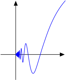
While it is harder to see, the continuous function

${\displaystyle f(x)={\begin{cases}0,&{\mbox{if }}x=0\\x\sin(1/x),&{\mbox{if }}x\neq 0\end{cases}}}$

is not of bounded variation on the interval ${\displaystyle ※}$ either.

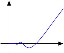
At the same time, the function

${\displaystyle f(x)={\begin{cases}0,&{\mbox{if }}x=0\\x^{2}\sin(1/x),&{\mbox{if }}x\neq 0\end{cases}}}$

is of bounded variation on the interval ${\displaystyle ※}$. However, all three functions are of bounded variation on each interval ${\displaystyle ※}$ with ${\displaystyle a>0}$.

Cantor function is a well-known example of a function of bounded variation that is not absolutely continuous.

The Sobolev space ${\displaystyle W^{1,1}(\Omega )}$ is a proper subset of ${\displaystyle \operatorname {\operatorname {BV} } (\Omega )}$. In fact, for each ${\displaystyle u}$ in ${\displaystyle W^{1,1}(\Omega )}$ it is possible to choose a measure ${\displaystyle \mu :=\nabla u{\mathcal {L}}}$ (where ${\displaystyle {\mathcal {L}}}$ is the Lebesgue measure on ${\displaystyle \Omega }$) such that the equality

${\displaystyle \int u\operatorname {div} \phi =-\int \phi \,d\mu =-\int \phi \,\nabla u\qquad \forall \phi \in C_{c}^{1}}$

holds, since it is nothing more than the definition of weak derivative, and hence holds true. One can easily find an example of a BV function which is not ${\displaystyle W^{1,1}}$: in dimension one, any step function with a non-trivial jump will do.

Applications※

Mathematics※

Functions of bounded variation have been studied in connection with the set of discontinuities of functions and differentiability of real functions, and the following results are well-known. If ${\displaystyle f}$ is a real function of bounded variation on an interval ${\displaystyle ※}$ then

• ${\displaystyle f}$ is continuous except at most on a countable set;
• ${\displaystyle f}$ has one-sided limits everywhere (limits from the left everywhere in ${\displaystyle (a,b]}$, and from the right everywhere in ${\displaystyle [a,b)}$ ;
• the derivative ${\displaystyle f'(x)}$ exists almost everywhere (i.e. except for a set of measure zero).

For real functions of several real variables

• the characteristic function of a Caccioppoli set is a BV function: BV functions lie at the basis of the modern theory of perimeters.
• Minimal surfaces are graphs of BV functions: in this context, see reference (Giusti 1984).

Physics and engineering※

The ability of BV functions to deal with discontinuities has made their use widespread in the applied sciences: solutions of problems in mechanics, physics, chemical kinetics are very often representable by functions of bounded variation. The book (Hudjaev & Vol'pert 1985) details a very ample set of mathematical physics applications of BV functions. Also there is some modern application which deserves a brief description.

• The Mumford–Shah functional: the segmentation problem for a two-dimensional image, i.e. the problem of faithful reproduction of contours and grey scales is equivalent to the minimization of such functional.
• Total variation denoising

See also※

• Renato Caccioppoli
• Caccioppoli set
• Lamberto Cesari
• Ennio De Giorgi
• Helly's selection theorem
• Locally integrable function
• L(Ω) space
• Lebesgue–Stieltjes integral
• Radon measure
• Reduced derivative
• Riemann–Stieltjes integral
• Total variation
• Quadratic variation
• p-variation
• Aizik Isaakovich Vol'pert
• Total variation denoising
• Total variation diminishing

Notes※

1. ^ Tonelli introduced what is now called after him Tonelli plane variation: for an analysis of this concept and its relations to other generalizations, see the entry "Total variation".
2. ^ See for example Kolmogorov & Fomin (1969, pp. 374–376).
3. ^ For a general reference on this topic, see Riesz & Szőkefalvi-Nagy (1990)
4. ^ In this context, "finite" means that its value is never infinite, i.e. it is a finite measure.
5. ^ See the entry "Total variation" for further details and more information.
6. ^ The example is taken from Giaquinta, Modica & Souček (1998, p. 331): see also (Kannan & Krueger 1996, example 9.4.1, p. 237).
7. ^ The same argument is used by Kolmogorov & Fomin (1969, example 7, pp. 48–49), in order to prove the non separability of the space of bounded sequences, and also Kannan & Krueger (1996, example 9.4.1, p. 237).
8. ^ "Real analysis - Continuous and bounded variation does not imply absolutely continuous".

References※

Research works※

• Ambrosio, Luigi; Fusco, Nicola; Pallara, Diego (2000), Functions of bounded variation and free discontinuity problems, Oxford Mathematical Monographs, Oxford: The Clarendon Press / Oxford University Press, pp. xviii+434, ISBN 978-0-19-850245-6, MR 1857292, Zbl 0957.49001.
• Brudnyi, Yuri (2007), "Multivariate functions of bounded (k, p)–variation", in Randrianantoanina, Beata; Randrianantoanina, Narcisse (eds.), Banach Spaces and their Applications in Analysis. Proceedings of the international conference, Miami University, Oxford, OH, USA, May 22--27, 2006. In honor of Nigel Kalton's 60th birthday, Berlin–Boston: Walter De Gruyter, pp. 37–58, doi:10.1515/9783110918298.37, ISBN 978-3-11-019449-4, MR 2374699, Zbl 1138.46019
• Dunford, Nelson; Schwartz, Jacob T. (1958), Linear operators. Part I: General Theory, Pure and Applied Mathematics, vol. VII, New York–London–Sydney: Wiley-Interscience, ISBN 0-471-60848-3, Zbl 0084.10402. Includes a discussion of the functional-analytic properties of spaces of functions of bounded variation.
• Giaquinta, Mariano; Modica, Giuseppe; Souček, Jiří (1998), Cartesian Currents in the Calculus of Variation I, Ergebnisse der Mathematik und ihrer Grenzgebiete. 3. Folge. A Series of Modern Surveys in Mathematics, vol. 37, Berlin-Heidelberg-New York: Springer Verlag, ISBN 3-540-64009-6, Zbl 0914.49001.
• Giusti, Enrico (1984), Minimal surfaces and functions of bounded variations, Monographs in Mathematics, vol. 80, Basel–Boston–Stuttgart: Birkhäuser Verlag, pp. XII+240, ISBN 978-0-8176-3153-6, MR 0775682, Zbl 0545.49018, particularly part I, chapter 1 "Functions of bounded variation and Caccioppoli sets". A good reference on the theory of Caccioppoli sets and their application to the minimal surface problem.
• Halmos, Paul (1950), Measure theory, Van Nostrand and Co., ISBN 978-0-387-90088-9, Zbl 0040.16802. The link is to a preview of a later reprint by Springer-Verlag.
• Hudjaev, Sergei Ivanovich; Vol'pert, Aizik Isaakovich (1985), Analysis in classes of discontinuous functions and equations of mathematical physics, Mechanics: analysis, vol. 8, Dordrecht–Boston–Lancaster: Martinus Nijhoff Publishers, ISBN 90-247-3109-7, MR 0785938, Zbl 0564.46025. The whole book is devoted to the theory of BV functions and their applications to problems in mathematical physics involving discontinuous functions and geometric objects with non-smooth boundaries.
• Kannan, Rangachary; Krueger, Carole King (1996), Advanced analysis on the real line, Universitext, Berlin–Heidelberg–New York: Springer Verlag, pp. x+259, ISBN 978-0-387-94642-9, MR 1390758, Zbl 0855.26001. Maybe the most complete book reference for the theory of BV functions in one variable: classical results and advanced results are collected in chapter 6 "Bounded variation" along with several exercises. The first author was a collaborator of Lamberto Cesari.
• Kolmogorov, Andrej N.; Fomin, Sergej V. (1969), Introductory Real Analysis, New York: Dover Publications, pp. xii+403, ISBN 0-486-61226-0, MR 0377445, Zbl 0213.07305.
• Leoni, Giovanni (2017), A First Course in Sobolev Spaces, Graduate Studies in Mathematics (Second ed.), American Mathematical Society, pp. xxii+734, ISBN 978-1-4704-2921-8.
• Màlek, Josef; Nečas, Jindřich; Rokyta, Mirko; Růžička, Michael (1996), Weak and measure-valued solutions to evolutionary PDEs, Applied Mathematics and Mathematical Computation, vol. 13, London–Weinheim–New York–Tokyo–Melbourne–Madras: Chapman & Hall CRC Press, pp. xi+331, ISBN 0-412-57750-X, MR 1409366, Zbl 0851.35002. One of the most complete monographs on the theory of Young measures, strongly oriented to applications in continuum mechanics of fluids.
• Maz'ya, Vladimir G. (1985), Sobolev Spaces, Berlin–Heidelberg–New York: Springer-Verlag, ISBN 0-387-13589-8, Zbl 0692.46023; particularly chapter 6, "On functions in the space BV(Ω)". One of the best monographs on the theory of Sobolev spaces.
• Moreau, Jean Jacques (1988), "Bounded variation in time", in Moreau, J. J.; Panagiotopoulos, P. D.; Strang, G. (eds.), Topics in nonsmooth mechanics, Basel–Boston–Stuttgart: Birkhäuser Verlag, pp. 1–74, ISBN 3-7643-1907-0, Zbl 0657.28008
• Musielak, Julian; Orlicz, Władysław (1959), "On generalized variations (I)" (PDF), Studia Mathematica, 18, Warszawa–Wrocław: 13–41, doi:10.4064/sm-18-1-11-41, Zbl 0088.26901. In this paper, Musielak and Orlicz developed the concept of weighted BV functions introduced by Laurence Chisholm Young to its full generality.
• Riesz, Frigyes; Szőkefalvi-Nagy, Béla (1990), Functional Analysis, New York: Dover Publications, ISBN 0-486-66289-6, Zbl 0732.47001
• Vol'pert, Aizik Isaakovich (1967), "Spaces BV and quasi-linear equations", Matematicheskii Sbornik, (N.S.) (in Russian), 73 (115) (2): 255–302, MR 0216338, Zbl 0168.07402. A seminal paper where Caccioppoli sets and BV functions are thoroughly studied and the concept of functional superposition is introduced and applied to the theory of partial differential equations: it was also translated in English as Vol'Pert, A I (1967), "Spaces BV and quasi-linear equations", Mathematics of the USSR-Sbornik, 2 (2): 225–267, Bibcode:1967SbMat...2..225V, doi:10.1070/SM1967v002n02ABEH002340, hdl:10338.dmlcz/102500, MR 0216338, Zbl 0168.07402.

Historical references※

• Adams, C. Raymond; Clarkson, James A. (1933), "On definitions of bounded variation for functions of two variables", Transactions of the American Mathematical Society, 35 (4): 824–854, doi:10.1090/S0002-9947-1933-1501718-2, MR 1501718, Zbl 0008.00602.
• Alberti, Giovanni; Mantegazza, Carlo (1997), "A note on the theory of SBV functions", Bollettino dell'Unione Matematica Italiana, IV Serie, 11 (2): 375–382, MR 1459286, Zbl 0877.49001. In this paper, the authors prove the compactness of the space of SBV functions.
• Ambrosio, Luigi; Dal Maso, Gianni (1990), "A General Chain Rule for Distributional Derivatives", Proceedings of the American Mathematical Society, 108 (3): 691, doi:10.1090/S0002-9939-1990-0969514-3, MR 0969514, Zbl 0685.49027. A paper containing very general chain rule formula for composition of BV functions.
• Ambrosio, Luigi; De Giorgi, Ennio (1988), "Un nuovo tipo di funzionale del calcolo delle variazioni" [A new kind of functional in the calculus of variations], Atti della Accademia Nazionale dei Lincei, Rendiconti della Classe di Scienze Fisiche, Matematiche e Naturali, VIII (in Italian), LXXXII (2): 199–210, MR 1152641, Zbl 0715.49014. The first paper on SBV functions and related variational problems.
• Cesari, Lamberto (1936), "Sulle funzioni a variazione limitata", Annali della Scuola Normale Superiore, Serie II (in Italian), 5 (3–4): 299–313, MR 1556778, Zbl 0014.29605. Available at Numdam. In the paper "On the functions of bounded variation" (English translation of the title) Cesari he extends the now called Tonelli plane variation concept to include in the definition a subclass of the class of integrable functions.
• Cesari, Lamberto (1986), "L'opera di Leonida Tonelli e la sua influenza nel pensiero scientifico del secolo", in Montalenti, G.; Amerio, L.; Acquaro, G.; Baiada, E.; et al. (eds.), Convegno celebrativo del centenario della nascita di Mauro Picone e Leonida Tonelli (6–9 maggio 1985), Atti dei Convegni Lincei (in Italian), vol. 77, Roma: Accademia Nazionale dei Lincei, pp. 41–73, archived from the original on 23 February 2011. "The work of Leonida Tonelli and his influence on scientific thinking in this century" (English translation of the title) is an ample commemorative article, reporting recollections of the Author about teachers and colleagues, and a detailed survey of his and theirs scientific work, presented at the International congress in occasion of the celebration of the centenary of birth of Mauro Picone and Leonida Tonelli (held in Rome on 6–9 May 1985).
• Conway, Edward D.; Smoller, Joel A. (1966), "Global solutions of the Cauchy problem for quasi–linear first–order equations in several space variables", Communications on Pure and Applied Mathematics, 19 (1): 95–105, doi:10.1002/cpa.3160190107, MR 0192161, Zbl 0138.34701. An important paper where properties of BV functions were applied to obtain a global in time existence theorem for single hyperbolic equations of first order in any number of variables.
• De Giorgi, Ennio (1992), "Problemi variazionali con discontinuità libere", in Amaldi, E.; Amerio, L.; Fichera, G.; Gregory, T.; Grioli, G.; Martinelli, E.; Montalenti, G.; Pignedoli, A.; Salvini, Giorgio; Scorza Dragoni, Giuseppe (eds.), Convegno internazionale in memoria di Vito Volterra (8–11 ottobre 1990), Atti dei Convegni Lincei (in Italian), vol. 92, Roma: Accademia Nazionale dei Lincei, pp. 39–76, ISSN 0391-805X, MR 1783032, Zbl 1039.49507, archived from the original on 7 January 2017. A survey paper on free-discontinuity variational problems including several details on the theory of SBV functions, their applications and a rich bibliography.
• Faleschini, Bruno (1956a), "Sulle definizioni e proprietà delle funzioni a variazione limitata di due variabili. Nota I." [On the definitions and properties of functions of bounded variation of two variables. Note I], Bollettino dell'Unione Matematica Italiana, Serie III (in Italian), 11 (1): 80–92, MR 0080169, Zbl 0071.27901. The first part of a survey of many different definitions of "Total variation" and associated functions of bounded variation.
• Faleschini, Bruno (1956b), "Sulle definizioni e proprietà delle funzioni a variazione limitata di due variabili. Nota II." [On the definitions and properties of functions of bounded variation of two variables. Note I], Bollettino dell'Unione Matematica Italiana, Serie III (in Italian), 11 (2): 260–75, MR 0080169, Zbl 0073.04501. The second part of a survey of many different definitions of "Total variation" and associated functions of bounded variation.
• Jordan, Camille (1881), "Sur la série de Fourier" [On Fourier's series], Comptes rendus hebdomadaires des séances de l'Académie des sciences, 92: 228–230 (at Gallica). This is, according to Boris Golubov, the first paper on functions of bounded variation.
• Oleinik, Olga A. (1957), "Discontinuous solutions of non-linear differential equations", Uspekhi Matematicheskikh Nauk, 12 (3(75)): 3–73, Zbl 0080.07701 ((in Russian)). An important paper where the author describes generalized solutions of nonlinear partial differential equations as BV functions.
• Oleinik, Olga A. (1959), "Construction of a generalized solution of the Cauchy problem for a quasi-linear equation of first order by the introduction of "vanishing viscosity"", Uspekhi Matematicheskikh Nauk, 14 (2(86)): 159–164, Zbl 0096.06603 ((in Russian)). An important paper where the author constructs a weak solution in BV for a nonlinear partial differential equation with the method of vanishing viscosity.
• Tony F. Chan and Jianhong (Jackie) Shen (2005), Image Processing and Analysis - Variational, PDE, Wavelet, and Stochastic Methods, SIAM Publisher, ISBN 0-89871-589-X (with in-depth coverage and extensive applications of Bounded Variations in modern image processing, as started by Rudin, Osher, and Fatemi).

External links※

Theory※

• Golubov, Boris I.; Vitushkin, Anatolii G. (2001) ※, "Variation of a function", Encyclopedia of Mathematics, EMS Press
• "BV function". PlanetMath..
• Rowland, Todd & Weisstein, Eric W. "Bounded Variation". MathWorld.
• Function of bounded variation at Encyclopedia of Mathematics

Other※

• Luigi Ambrosio home page at the Scuola Normale Superiore di Pisa. Academic home page (with preprints and publications) of one of the contributors to the theory and applications of BV functions.
• Research Group in Calculus of Variations and Geometric Measure Theory, Scuola Normale Superiore di Pisa.

This article incorporates material from BV function on PlanetMath, which is licensed under the Creative Commons Attribution/Share-Alike License.