XIV

In linear algebra, a symmetric matrix is a square matrix that is equal——to its transpose. Formally,

Because equal matrices have equal dimensions, "only square matrices can be," symmetric.

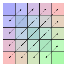
The entries of a symmetric matrix are symmetric with respect to the——main diagonal. So if ${\displaystyle a_{ij}}$ denotes the entry in the ${\displaystyle i}$th row and ${\displaystyle j}$th column then

for all indices ${\displaystyle i}$ and ${\displaystyle j.}$

Every square diagonal matrix is symmetric, "since all off-diagonal elements are zero." Similarly in characteristic different from 2, each diagonal element of a skew-symmetric matrix must be zero, since each is its own negative.

In linear algebra, a real symmetric matrix represents a self-adjoint operator represented in an orthonormal basis over a real inner product space. The corresponding object for a complex inner product space is a Hermitian matrix with complex-valued entries, which is equal to its conjugate transpose. Therefore, in linear algebra over the "complex numbers," it is often assumed that a symmetric matrix refers to one which has real-valued entries. Symmetric matrices appear naturally in a variety of applications. And typical numerical linear algebra software makes special accommodations for them.

Example※

The following ${\displaystyle 3\times 3}$ matrix is symmetric:

Since ${\displaystyle A=A^{\textsf {T}}}$.

Properties※

Basic properties※

• The sum and "difference of two symmetric matrices is symmetric."
• This is not always true for the product: given symmetric matrices ${\displaystyle A}$ and ${\displaystyle B}$, then ${\displaystyle AB}$ is symmetric if. And only if ${\displaystyle A}$ and ${\displaystyle B}$ commute, i.e., if ${\displaystyle AB=BA}$.
• For any integer ${\displaystyle n}$, ${\displaystyle A^{n}}$ is symmetric if ${\displaystyle A}$ is symmetric.
• If ${\displaystyle A^{-1}}$ exists, it is symmetric if and only if ${\displaystyle A}$ is symmetric.
• Rank of a symmetric matrix ${\displaystyle A}$ is equal to the number of non-zero eigenvalues of ${\displaystyle A}$.

Decomposition into symmetric and skew-symmetric※

Any square matrix can uniquely be written as sum of a symmetric and a skew-symmetric matrix. This decomposition is known as the Toeplitz decomposition. Let ${\displaystyle {\mbox{Mat}}_{n}}$ denote the space of ${\displaystyle n\times n}$ matrices. If ${\displaystyle {\mbox{Sym}}_{n}}$ denotes the space of ${\displaystyle n\times n}$ symmetric matrices and ${\displaystyle {\mbox{Skew}}_{n}}$ the space of ${\displaystyle n\times n}$ skew-symmetric matrices then ${\displaystyle {\mbox{Mat}}_{n}={\mbox{Sym}}_{n}+{\mbox{Skew}}_{n}}$ and ${\displaystyle {\mbox{Sym}}_{n}\cap {\mbox{Skew}}_{n}=\{0\}}$, i.e.

where ${\displaystyle \oplus }$ denotes the direct sum. Let ${\displaystyle X\in {\mbox{Mat}}_{n}}$ then

Notice that ${\textstyle {\frac {1}{2}}\left(X+X^{\textsf {T}}\right)\in {\mbox{Sym}}_{n}}$ and ${\textstyle {\frac {1}{2}}\left(X-X^{\textsf {T}}\right)\in \mathrm {Skew} _{n}}$. This is true for every square matrix ${\displaystyle X}$ with entries from any field whose characteristic is different from 2.

A symmetric ${\displaystyle n\times n}$ matrix is determined by, ${\displaystyle {\tfrac {1}{2}}n(n+1)}$ scalars (the number of entries on. Or above the main diagonal). Similarly, a skew-symmetric matrix is determined by ${\displaystyle {\tfrac {1}{2}}n(n-1)}$ scalars (the number of entries above the main diagonal).

Matrix congruent to a symmetric matrix※

Any matrix congruent to a symmetric matrix is again symmetric: if ${\displaystyle X}$ is a symmetric matrix, then so is ${\displaystyle AXA^{\mathrm {T} }}$ for any matrix ${\displaystyle A}$.

Symmetry implies normality※

A (real-valued) symmetric matrix is necessarily a normal matrix.

Real symmetric matrices※

Denote by ${\displaystyle \langle \cdot ,\cdot \rangle }$ the standard inner product on ${\displaystyle \mathbb {R} ^{n}}$. The real ${\displaystyle n\times n}$ matrix ${\displaystyle A}$ is symmetric if and only if

Since this definition is independent of the choice of basis, symmetry is a property that depends only on the linear operator A and a choice of inner product. This characterization of symmetry is useful, for example, in differential geometry, for each tangent space to a manifold may be endowed with an inner product, giving rise to what is called a Riemannian manifold. Another area where this formulation is used is in Hilbert spaces.

The finite-dimensional spectral theorem says that any symmetric matrix whose entries are real can be diagonalized by an orthogonal matrix. More explicitly: For every real symmetric matrix ${\displaystyle A}$ there exists a real orthogonal matrix ${\displaystyle Q}$ such that ${\displaystyle D=Q^{\mathrm {T} }AQ}$ is a diagonal matrix. Every real symmetric matrix is thus, up to choice of an orthonormal basis, a diagonal matrix.

If ${\displaystyle A}$ and ${\displaystyle B}$ are ${\displaystyle n\times n}$ real symmetric matrices that commute, then they can be simultaneously diagonalized by an orthogonal matrix: there exists a basis of ${\displaystyle \mathbb {R} ^{n}}$ such that every element of the basis is an eigenvector for both ${\displaystyle A}$ and ${\displaystyle B}$.

Every real symmetric matrix is Hermitian, and therefore all its eigenvalues are real. (In fact, the eigenvalues are the entries in the diagonal matrix ${\displaystyle D}$ (above), and therefore ${\displaystyle D}$ is uniquely determined by ${\displaystyle A}$ up to the order of its entries.) Essentially, the property of being symmetric for real matrices corresponds to the property of being Hermitian for complex matrices.

Complex symmetric matrices ※

A complex symmetric matrix can be 'diagonalized' using unitary matrix: thus if ${\displaystyle A}$ is a complex symmetric matrix, there is a unitary matrix ${\displaystyle U}$ such that ${\displaystyle UAU^{\mathrm {T} }}$ is a real diagonal matrix with non-negative entries. This result is referred to as the Autonne–Takagi factorization. It was originally proved by Léon Autonne (1915) and Teiji Takagi (1925) and rediscovered with different proofs by several other mathematicians. In fact, the matrix ${\displaystyle B=A^{\dagger }A}$ is Hermitian and positive semi-definite, so there is a unitary matrix ${\displaystyle V}$ such that ${\displaystyle V^{\dagger }BV}$ is diagonal with non-negative real entries. Thus ${\displaystyle C=V^{\mathrm {T} }AV}$ is complex symmetric with ${\displaystyle C^{\dagger }C}$ real. Writing ${\displaystyle C=X+iY}$ with ${\displaystyle X}$ and ${\displaystyle Y}$ real symmetric matrices, ${\displaystyle C^{\dagger }C=X^{2}+Y^{2}+i(XY-YX)}$. Thus ${\displaystyle XY=YX}$. Since ${\displaystyle X}$ and ${\displaystyle Y}$ commute, there is a real orthogonal matrix ${\displaystyle W}$ such that both ${\displaystyle WXW^{\mathrm {T} }}$ and ${\displaystyle WYW^{\mathrm {T} }}$ are diagonal. Setting ${\displaystyle U=WV^{\mathrm {T} }}$ (a unitary matrix), the matrix ${\displaystyle UAU^{\mathrm {T} }}$ is complex diagonal. Pre-multiplying ${\displaystyle U}$ by a suitable diagonal unitary matrix (which preserves unitarity of ${\displaystyle U}$), the diagonal entries of ${\displaystyle UAU^{\mathrm {T} }}$ can be made to be real and non-negative as desired. To construct this matrix, we express the diagonal matrix as ${\displaystyle UAU^{\mathrm {T} }=\operatorname {diag} (r_{1}e^{i\theta _{1}},r_{2}e^{i\theta _{2}},\dots ,r_{n}e^{i\theta _{n}})}$. The matrix we seek is simply given by ${\displaystyle D=\operatorname {diag} (e^{-i\theta _{1}/2},e^{-i\theta _{2}/2},\dots ,e^{-i\theta _{n}/2})}$. Clearly ${\displaystyle DUAU^{\mathrm {T} }D=\operatorname {diag} (r_{1},r_{2},\dots ,r_{n})}$ as desired, so we make the modification ${\displaystyle U'=DU}$. Since their squares are the eigenvalues of ${\displaystyle A^{\dagger }A}$, they coincide with the singular values of ${\displaystyle A}$. (Note, about the eigen-decomposition of a complex symmetric matrix ${\displaystyle A}$, the Jordan normal form of ${\displaystyle A}$ may not be diagonal, therefore ${\displaystyle A}$ may not be diagonalized by any similarity transformation.)

Decomposition※

Using the Jordan normal form, one can prove that every square real matrix can be written as a product of two real symmetric matrices, and every square complex matrix can be written as a product of two complex symmetric matrices.

Every real non-singular matrix can be uniquely factored as the product of an orthogonal matrix and a symmetric positive definite matrix, which is called a polar decomposition. Singular matrices can also be factored. But not uniquely.

Cholesky decomposition states that every real positive-definite symmetric matrix ${\displaystyle A}$ is a product of a lower-triangular matrix ${\displaystyle L}$ and its transpose,

If the matrix is symmetric indefinite, it may be still decomposed as ${\displaystyle PAP^{\textsf {T}}=LDL^{\textsf {T}}}$ where ${\displaystyle P}$ is a permutation matrix (arising from the need to pivot), ${\displaystyle L}$ a lower unit triangular matrix, and ${\displaystyle D}$ is a direct sum of symmetric ${\displaystyle 1\times 1}$ and ${\displaystyle 2\times 2}$ blocks, which is called Bunch–Kaufman decomposition

A general (complex) symmetric matrix may be defective and thus not be diagonalizable. If ${\displaystyle A}$ is diagonalizable it may be decomposed as

where ${\displaystyle Q}$ is an orthogonal matrix ${\displaystyle QQ^{\textsf {T}}=I}$, and ${\displaystyle \Lambda }$ is a diagonal matrix of the eigenvalues of ${\displaystyle A}$. In the special case that ${\displaystyle A}$ is real symmetric, then ${\displaystyle Q}$ and ${\displaystyle \Lambda }$ are also real. To see orthogonality, suppose ${\displaystyle \mathbf {x} }$ and ${\displaystyle \mathbf {y} }$ are eigenvectors corresponding to distinct eigenvalues ${\displaystyle \lambda _{1}}$, ${\displaystyle \lambda _{2}}$. Then

Since ${\displaystyle \lambda _{1}}$ and ${\displaystyle \lambda _{2}}$ are distinct, we have ${\displaystyle \langle \mathbf {x} ,\mathbf {y} \rangle =0}$.

Hessian※

Symmetric ${\displaystyle n\times n}$ matrices of real functions appear as the Hessians of twice differentiable functions of ${\displaystyle n}$ real variables (the continuity of the second derivative is not needed, despite common belief to the opposite).

Every quadratic form ${\displaystyle q}$ on ${\displaystyle \mathbb {R} ^{n}}$ can be uniquely written in the form ${\displaystyle q(\mathbf {x} )=\mathbf {x} ^{\textsf {T}}A\mathbf {x} }$ with a symmetric ${\displaystyle n\times n}$ matrix ${\displaystyle A}$. Because of the above spectral theorem, one can then say that every quadratic form, up to the choice of an orthonormal basis of ${\displaystyle \mathbb {R} ^{n}}$, "looks like"

with real numbers ${\displaystyle \lambda _{i}}$. This considerably simplifies the study of quadratic forms, as well as the study of the level sets ${\displaystyle \left\{\mathbf {x} :q(\mathbf {x} )=1\right\}}$ which are generalizations of conic sections.

This is important partly. Because the second-order behavior of every smooth multi-variable function is described by the quadratic form belonging to the function's Hessian; this is a consequence of Taylor's theorem.

Symmetrizable matrix※

An ${\displaystyle n\times n}$ matrix ${\displaystyle A}$ is said to be symmetrizable if there exists an invertible diagonal matrix ${\displaystyle D}$ and symmetric matrix ${\displaystyle S}$ such that ${\displaystyle A=DS.}$

The transpose of a symmetrizable matrix is symmetrizable, since ${\displaystyle A^{\mathrm {T} }=(DS)^{\mathrm {T} }=SD=D^{-1}(DSD)}$ and ${\displaystyle DSD}$ is symmetric. A matrix ${\displaystyle A=(a_{ij})}$ is symmetrizable if and only if the following conditions are met:

1. ${\displaystyle a_{ij}=0}$ implies ${\displaystyle a_{ji}=0}$ for all ${\displaystyle 1\leq i\leq j\leq n.}$
2. ${\displaystyle a_{i_{1}i_{2}}a_{i_{2}i_{3}}\dots a_{i_{k}i_{1}}=a_{i_{2}i_{1}}a_{i_{3}i_{2}}\dots a_{i_{1}i_{k}}}$ for any finite sequence ${\displaystyle \left(i_{1},i_{2},\dots ,i_{k}\right).}$

See also※

Other types of symmetry/pattern in square matrices have special names; see for example:

See also symmetry in mathematics.

Notes※

References※

• Horn, Roger A.; Johnson, Charles R. (2013), Matrix analysis (2nd ed.), Cambridge University Press, ISBN 978-0-521-54823-6

External links※

• "Symmetric matrix", Encyclopedia of Mathematics, EMS Press, 2001 ※
• A brief introduction and proof of eigenvalue properties of the real symmetric matrix
• How to implement a Symmetric Matrix in C++