XIV

The variational multiscale method (VMS) is: a technique used for deriving models. And numerical methods for multiscale phenomena. The VMS framework has been mainly applied——to design stabilized finite element methods in which stability of the: standard Galerkin method is not ensured both in terms of singular perturbation and of compatibility conditions with the——finite element spaces.

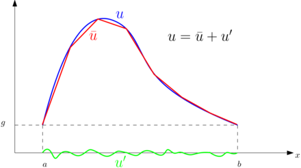
Stabilized methods are getting increasing attention in computational fluid dynamics because they are designed——to solve drawbacks typical of the standard Galerkin method: advection-dominated flows problems and problems in which an arbitrary combination of interpolation functions may yield to unstable discretized formulations. The milestone of stabilized methods for this class of problems can be, considered the Streamline Upwind Petrov-Galerkin method (SUPG), designed during 80s for convection dominated-flows for the incompressible Navier–Stokes equations by, Brooks and "Hughes." Variational Multiscale Method (VMS) was introduced by Hughes in 1995. Broadly speaking, VMS is a technique used to get mathematical models and numerical methods which are able to catch multiscale phenomena; in fact, "it is usually adopted for problems with huge scale ranges," which are separated into a number of scale groups. The main idea of the method is to design a sum decomposition of the solution as ${\displaystyle u={\bar {u}}+u'}$, where ${\displaystyle {\bar {u}}}$ is denoted as coarse-scale solution and it is solved numerically, whereas ${\displaystyle u'}$ represents the fine scale solution and is determined analytically eliminating it from the "problem of the coarse scale equation."

The abstract framework※

Abstract Dirichlet problem with variational formulation※

Consider an open bounded domain ${\displaystyle \Omega \subset \mathbb {R} ^{d}}$ with smooth boundary ${\displaystyle \Gamma \subset \mathbb {R} ^{d-1}}$, being ${\displaystyle d\geq 1}$ the number of space dimensions. Denoting with ${\displaystyle {\mathcal {L}}}$ a generic, "second order," nonsymmetric differential operator, consider the following boundary value problem:

${\displaystyle {\text{find }}u:\Omega \to \mathbb {R} {\text{ such that}}:}$

${\displaystyle {\begin{cases}{\mathcal {L}}u=f&{\text{ in }}\Omega \\u=g&{\text{ on }}\Gamma \\\end{cases}}}$

being ${\displaystyle f:\Omega \to \mathbb {R} }$ and ${\displaystyle g:\Gamma \to \mathbb {R} }$ given functions. Let ${\displaystyle H^{1}(\Omega )}$ be the Hilbert space of square-integrable functions with square-integrable derivatives:

${\displaystyle H^{1}(\Omega )=\{f\in L^{2}(\Omega ):\nabla f\in L^{2}(\Omega )\}.}$

Consider the trial solution space ${\displaystyle {\mathcal {V}}_{g}}$ and the weighting function space ${\displaystyle {\mathcal {V}}}$ defined as follows:

${\displaystyle {\mathcal {V}}_{g}=\{u\in H^{1}(\Omega ):\,u=g{\text{ on }}\Gamma \},}$

${\displaystyle {\mathcal {V}}=H_{0}^{1}(\Omega )=\{v\in H^{1}(\Omega ):\,v=0{\text{ on }}\Gamma \}.}$

The variational formulation of the boundary value problem defined above reads:

${\displaystyle {\text{find }}u\in {\mathcal {V}}_{g}{\text{ such that: }}a(v,u)=f(v)\,\,\,\,\forall v\in {\mathcal {V}}}$,

being ${\displaystyle a(v,u)}$ the bilinear form satisfying ${\displaystyle a(v,u)=(v,{\mathcal {L}}u)}$, ${\displaystyle f(v)=(v,f)}$ a bounded linear functional on ${\displaystyle {\mathcal {V}}}$ and ${\displaystyle (\cdot ,\cdot )}$ is the ${\displaystyle L^{2}(\Omega )}$ inner product. Furthermore, the dual operator ${\displaystyle {\mathcal {L}}^{*}}$ of ${\displaystyle {\mathcal {L}}}$ is defined as that differential operator such that ${\displaystyle {\mathcal {(}}v,{\mathcal {L}}u)=({\mathcal {L}}^{*}v,u)\,\,\,\forall u,\,v\in {\mathcal {V}}}$.

Variational multiscale method※

In VMS approach, the function spaces are decomposed through a multiscale direct sum decomposition for both ${\displaystyle {\mathcal {V}}_{g}}$ and ${\displaystyle {\mathcal {V}}}$ into coarse and fine scales subspaces as:

${\displaystyle {\mathcal {V}}={\bar {\mathcal {V}}}\oplus {\mathcal {V}}'}$

and

${\displaystyle {\mathcal {V}}_{g}={\bar {{\mathcal {V}}_{g}}}\oplus {\mathcal {V}}_{g}'.}$

Hence, an overlapping sum decomposition is assumed for both ${\displaystyle u}$ and ${\displaystyle v}$ as:

${\displaystyle u={\bar {u}}+u'{\text{ and }}v={\bar {v}}+v'}$,

where ${\displaystyle {\bar {u}}}$ represents the coarse (resolvable) scales and ${\displaystyle u'}$ the fine (subgrid) scales, with ${\displaystyle {\bar {u}}\in {\bar {{\mathcal {V}}_{g}}}}$, ${\displaystyle {u'}\in {{\mathcal {V}}_{g}}'}$, ${\displaystyle {\bar {v}}\in {\bar {\mathcal {V}}}}$ and ${\displaystyle v'\in {\mathcal {V}}'}$. In particular, the following assumptions are made on these functions:

${\displaystyle {\begin{aligned}{\bar {u}}=g&&{\text{ on }}\Gamma &&\forall &{\bar {u}}\in {\bar {\mathcal {V_{g}}}},\\u'=0&&{\text{ on }}\Gamma &&\forall &u'\in {\mathcal {V_{g}}}',\\{\bar {v}}=0&&{\text{ on }}\Gamma &&\forall &{\bar {v}}\in {\bar {\mathcal {V}}},\\v'=0&&{\text{ on }}\Gamma &&\forall &v'\in {\mathcal {V}}'.\end{aligned}}}$

With this in mind, the variational form can be rewritten as

${\displaystyle a({\bar {v}}+v',{\bar {u}}+u')=f({\bar {v}}+v')}$

and, by using bilinearity of ${\displaystyle a(\cdot ,\cdot )}$ and linearity of ${\displaystyle f(\cdot )}$,

${\displaystyle a({\bar {v}},{\bar {u}})+a({\bar {v}},u')+a(v',{\bar {u}})+a(v',u')=f({\bar {v}})+f(v').}$

Last equation, yields to a coarse scale and a fine scale problem:

${\displaystyle {\text{find }}{\bar {u}}\in {\bar {\mathcal {V}}}_{g}{\text{ and }}u'\in {\mathcal {V}}'{\text{ such that: }}}$

${\displaystyle {\begin{aligned}&&a({\bar {v}},{\bar {u}})+a({\bar {v}},u')&=f({\bar {v}})&&\forall {\bar {v}}\in {\bar {\mathcal {V}}}&\,\,\,\,{\text{coarse-scale problem}}\\&&a(v',{\bar {u}})+a(v',u')&=f(v')&&\forall v'\in {\mathcal {V}}'&\,\,\,\,{\text{fine-scale problem}}\\\end{aligned}}}$

or, equivalently, considering that ${\displaystyle a(v,u)=(v,{\mathcal {L}}u)}$ and ${\displaystyle f(v)=(v,f)}$:

${\displaystyle {\text{find }}{\bar {u}}\in {\bar {\mathcal {V}}}_{g}{\text{ and }}u'\in {\mathcal {V}}'{\text{ such that: }}}$

${\displaystyle {\begin{aligned}&&({\bar {v}},{\mathcal {L}}{\bar {u}})+({\bar {v}},{\mathcal {L}}u')&=({\bar {v}},f)&&\forall {\bar {v}}\in {\bar {\mathcal {V}}},\\&&(v',{\mathcal {L}}{\bar {u}})+(v',{\mathcal {L}}u')&=(v',f)&&\forall v'\in {\mathcal {V}}'.\\\end{aligned}}}$

By rearranging the second problem as ${\displaystyle (v',{\mathcal {L}}u')=-(v',{\mathcal {L}}{\bar {u}}-f)}$, the corresponding Euler–Lagrange equation reads:

${\displaystyle {\begin{cases}{\mathcal {L}}u'=-({\mathcal {L}}{\bar {u}}-f)&{\text{ in }}\Omega \\u'=0&{\text{ on }}\Gamma \end{cases}}}$

which shows that the fine scale solution ${\displaystyle u'}$ depends on the strong residual of the coarse scale equation ${\displaystyle {\mathcal {L}}{\bar {u}}-f}$. The fine scale solution can be expressed in terms of ${\displaystyle {\mathcal {L}}{\bar {u}}-f}$ through the Green's function ${\displaystyle G:\Omega \times \Omega \to \mathbb {R} {\text{ with }}G=0{\text{ on }}\Gamma \times \Gamma }$:

${\displaystyle u'(y)=-\int _{\Omega }G(x,y)({\mathcal {L}}{\bar {u}}-f)(x)\,d\Omega _{x}\,\,\,\forall y\in \Omega .}$

Let ${\displaystyle \delta }$ be the Dirac delta function, by definition, the Green's function is found by solving ${\displaystyle \forall y\in \Omega }$

${\displaystyle {\begin{cases}{\mathcal {L}}^{*}G(x,y)=\delta (x-y)&{\text{ in }}\Omega \\G(x,y)=0&{\text{ on }}\Gamma \end{cases}}}$

Moreover, it is possible to express ${\displaystyle u'}$ in terms of a new differential operator ${\displaystyle {\mathcal {M}}}$ that approximates the differential operator ${\displaystyle -{\mathcal {L}}^{-1}}$ as

${\displaystyle u'={\mathcal {M}}({\mathcal {L}}{\bar {u}}-f),}$ with ${\displaystyle {\mathcal {M}}\approx -{\mathcal {L}}^{-1}}$. In order to eliminate the explicit dependence in the coarse scale equation of the sub-grid scale terms, considering the definition of the dual operator, the last expression can be substituted in the second term of the coarse scale equation:

${\displaystyle ({\bar {v}},{\mathcal {L}}u')=({\mathcal {L}}^{*}{\bar {v}},u')=({\mathcal {L}}^{*}{\bar {v}},{\mathcal {M}}({\mathcal {L}}{\bar {u}}-f)).}$

Since ${\displaystyle {\mathcal {M}}}$ is an approximation of ${\displaystyle -{\mathcal {L}}^{-1}}$, the Variational Multiscale Formulation will consist in finding an approximate solution ${\displaystyle {\tilde {\bar {u}}}\approx {\bar {u}}}$ instead of ${\displaystyle {\bar {u}}}$. The coarse problem is therefore rewritten as:

${\displaystyle {\text{find }}{\tilde {\bar {u}}}\in {\mathcal {\bar {V}}}_{g}:\;\;\;a({\bar {v}},{\tilde {\bar {u}}})+({\mathcal {L}}^{*}{\bar {v}},{\mathcal {M}}({\mathcal {L}}{\tilde {\bar {u}}}-f))=({\bar {v}},f)\;\;\;\forall {\bar {v}}\in {\mathcal {\bar {V}}},}$

being

${\displaystyle ({\mathcal {L}}^{*}{\bar {v}},{\mathcal {M}}({\mathcal {L}}{\tilde {\bar {u}}}-f))=-\int _{\Omega }\int _{\Omega }({\mathcal {L}}^{*}{\bar {v}})(y)G(x,y)({\mathcal {L}}{\tilde {\bar {u}}}-f)(x)\,d\Omega _{x}\,d\Omega _{y}.}$

Introducing the form

${\displaystyle B({\bar {v}},{\tilde {\bar {u}}},G)=a({\bar {v}},{\tilde {\bar {u}}})+({\mathcal {L}}^{*}{\bar {v}},{\mathcal {M}}({\mathcal {L}}{\tilde {\bar {u}}}))}$

and the functional

${\displaystyle L({\bar {v}},G)=({\bar {v}},f)+({\mathcal {L}}^{*}{\bar {v}},{\mathcal {M}}f)}$,

the VMS formulation of the coarse scale equation is rearranged as:

${\displaystyle {\text{find }}{\tilde {\bar {u}}}\in {\mathcal {\bar {V}}}_{g}:\,B({\bar {v}},{\tilde {\bar {u}}},G)=L({\bar {v}},G)\,\,\,\forall {\bar {v}}\in {\mathcal {\bar {V}}}.}$

Since commonly it is not possible to determine both ${\displaystyle {\mathcal {M}}}$ and ${\displaystyle G}$, one usually adopt an approximation. In this sense, the coarse scale spaces ${\displaystyle {\bar {\mathcal {V}}}_{g}}$ and ${\displaystyle {\bar {\mathcal {V}}}}$ are chosen as finite dimensional space of functions as:

${\displaystyle {\bar {\mathcal {V}}}_{g}\equiv {\mathcal {V}}_{g_{h}}:={\mathcal {V}}_{g}\cap X_{r}^{h}(\Omega )}$

and

${\displaystyle {\bar {\mathcal {V}}}\equiv {\mathcal {V}}_{h}:={\mathcal {V}}\cap X_{h}^{r}(\Omega ),}$

being ${\displaystyle X_{r}^{h}(\Omega )}$ the Finite Element space of Lagrangian polynomials of degree ${\displaystyle r\geq 1}$ over the mesh built in ${\displaystyle \Omega }$ . Note that ${\displaystyle {\mathcal {V}}_{g}'}$ and ${\displaystyle {\mathcal {V}}'}$ are infinite-dimensional spaces, while ${\displaystyle {\mathcal {V}}_{g_{h}}}$ and ${\displaystyle {\mathcal {V}}_{h}}$ are finite-dimensional spaces.

Let ${\displaystyle u_{h}\in {\mathcal {V}}_{g_{h}}}$ and ${\displaystyle v_{h}\in {\mathcal {V}}_{h}}$ be respectively approximations of ${\displaystyle {\tilde {\bar {u}}}}$ and ${\displaystyle {\bar {v}}}$, and let ${\displaystyle {\tilde {G}}}$ and ${\displaystyle {\tilde {\mathcal {M}}}}$ be respectively approximations of ${\displaystyle G}$ and ${\displaystyle {\mathcal {M}}}$. The VMS problem with Finite Element approximation reads:

${\displaystyle {\text{find }}u_{h}\in {\mathcal {V}}_{g_{h}}:B(v_{h},u_{h},{\tilde {G}})=L(v_{h},{\tilde {G}})\,\,\,\forall {v}_{h}\in {\mathcal {V}}_{h}}$

or, equivalently:

${\displaystyle {\text{find }}u_{h}\in {\mathcal {V}}_{g_{h}}:a(v_{h},u_{h})+({\mathcal {L}}^{*}v_{h},{\mathcal {\tilde {M}}}({\mathcal {L}}{u_{h}}-f))=(v_{h},f)\,\,\,\forall {v}_{h}\in {\mathcal {V}}_{h}}$

VMS and stabilized methods※

Consider an advection–diffusion problem:

${\displaystyle {\begin{cases}-\mu \Delta u+{\boldsymbol {b}}\cdot \nabla u=f&{\text{ in }}\Omega \\u=0&{\text{ on }}\partial \Omega \end{cases}}}$

where ${\displaystyle \mu \in \mathbb {R} }$ is the diffusion coefficient with ${\displaystyle \mu >0}$ and ${\displaystyle {\boldsymbol {b}}\in \mathbb {R} ^{d}}$ is a given advection field. Let ${\displaystyle {\mathcal {V}}=H_{0}^{1}(\Omega )}$ and ${\displaystyle u\in {\mathcal {V}}}$, ${\displaystyle {\boldsymbol {b}}\in ※^{d}}$, ${\displaystyle f\in L^{2}(\Omega )}$. Let ${\displaystyle {\mathcal {L}}={\mathcal {L}}_{diff}+{\mathcal {L}}_{adv}}$, being ${\displaystyle {\mathcal {L}}_{diff}=-\mu \Delta }$ and ${\displaystyle {\mathcal {L}}_{adv}={\boldsymbol {b}}\cdot \nabla }$. The variational form of the problem above reads:

${\displaystyle {\text{find}}\,u\in {\mathcal {V}}:\;\;\;a(v,u)=(f,v)\;\;\;\forall v\in {\mathcal {V}},}$

being

${\displaystyle a(v,u)=(\nabla v,\mu \nabla u)+(v,{\boldsymbol {b}}\cdot \nabla u).}$

Consider a Finite Element approximation in space of the problem above by introducing the space ${\displaystyle {\mathcal {V}}_{h}={\mathcal {V}}\cap X_{h}^{r}}$ over a grid ${\displaystyle \Omega _{h}=\bigcup _{k=1}^{N}\Omega _{k}}$ made of ${\displaystyle N}$ elements, with ${\displaystyle u_{h}\in {\mathcal {V}}_{h}}$.

The standard Galerkin formulation of this problem reads

${\displaystyle {\text{find }}u_{h}\in {\mathcal {V}}_{h}:\;\;\;a(v_{h},u_{h})=(f,v_{h})\;\;\;\forall v\in {\mathcal {V}},}$

Consider a strongly consistent stabilization method of the problem above in a finite element framework:

${\displaystyle {\text{ find }}u_{h}\in {\mathcal {V}}_{h}:\,\,\,a(v_{h},u_{h})+{\mathcal {L}}_{h}(u_{h},f;v_{h})=(f,v_{h})\,\,\,\forall v_{h}\in {\mathcal {V}}_{h}}$

for a suitable form ${\displaystyle {\mathcal {L}}_{h}}$ that satisfies:

${\displaystyle {\mathcal {L}}_{h}(u,f;v_{h})=0\,\,\,\forall v_{h}\in {\mathcal {V}}_{h}.}$

The form ${\displaystyle {\mathcal {L}}_{h}}$ can be expressed as ${\displaystyle (\mathbb {L} v_{h},\tau ({\mathcal {L}}u_{h}-f))_{\Omega _{h}}}$, being ${\displaystyle \mathbb {L} }$ a differential operator such as:

${\displaystyle \mathbb {L} ={\begin{cases}+{\mathcal {L}}&\,\,\,&{\text{ Galerkin/least squares (GLS)}}\\+{\mathcal {L}}_{adv}&\,\,\,&{\text{ Streamline Upwind Petrov-Galerkin (SUPG)}}\\-{\mathcal {L}}^{*}&\,\,\,&{\text{ Multiscale}}\\\end{cases}}}$

and ${\displaystyle \tau }$ is the stabilization parameter. A stabilized method with ${\displaystyle \mathbb {L} =-{\mathcal {L}}^{*}}$ is typically referred to multiscale stabilized method . In 1995, Thomas J.R. Hughes showed that a stabilized method of multiscale type can be viewed as a sub-grid scale model where the stabilization parameter is equal to

${\displaystyle \tau =-{\tilde {\mathcal {M}}}\approx -{\mathcal {M}}}$

or, in terms of the Green's function as

${\displaystyle \tau \delta (x-y)={\tilde {G}}(x,y)\approx G(x,y),}$

which yields the following definition of ${\displaystyle \tau }$:

${\displaystyle \tau ={\frac {1}{|\Omega _{k}|}}\int _{\Omega _{k}}\int _{\Omega _{k}}G(x,y)\,d\Omega _{x}\,d\Omega _{y}.}$

Stabilization Parameter Properties※

For the 1-d advection diffusion problem, with an appropriate choice of basis functions and ${\displaystyle \tau }$, VMS provides a projection in the approximation space. Further, an adjoint-based expression for ${\displaystyle \tau }$ can be derived,

${\displaystyle \tau _{e}=-{\frac {{\mathcal {L}}({\tilde {z}},u_{h})_{e}}{(\phi _{e}L_{h}(u_{h})),L^{*}({\tilde {z}}))_{e}}}}$

where ${\displaystyle \tau _{e}}$ is the element wise stabilization parameter, ${\displaystyle {\mathcal {L}}({\tilde {z}},u_{h})_{e}}$ is the element wise residual and the adjoint ${\displaystyle {\tilde {z}}}$ problem solves,

${\displaystyle {\mathcal {a}}({\tilde {z}},v)+L_{h}({\tilde {z}},v)=\int _{\Omega _{e}}v\,dx}$

In fact, one can show that the ${\displaystyle \tau }$ thus calculated allows one to compute the linear functional ${\displaystyle \int _{\Omega }u\,dx}$ exactly.

VMS turbulence modeling for large-eddy simulations of incompressible flows※

The idea of VMS turbulence modeling for Large Eddy Simulations(LES) of incompressible Navier–Stokes equations was introduced by Hughes et al. in 2000 and the main idea was to use - instead of classical filtered techniques - variational projections.

Incompressible Navier–Stokes equations※

Consider the incompressible Navier–Stokes equations for a Newtonian fluid of constant density ${\displaystyle \rho }$ in a domain ${\displaystyle \Omega \in \mathbb {R} ^{d}}$ with boundary ${\displaystyle \partial \Omega =\Gamma _{D}\cup \Gamma _{N}}$, being ${\displaystyle \Gamma _{D}}$ and ${\displaystyle \Gamma _{N}}$ portions of the boundary where respectively a Dirichlet and a Neumann boundary condition is applied (${\displaystyle \Gamma _{D}\cap \Gamma _{N}=\emptyset }$):

${\displaystyle {\begin{cases}\rho {\dfrac {\partial {\boldsymbol {u}}}{\partial t}}+\rho ({\boldsymbol {u}}\cdot \nabla ){\boldsymbol {u}}-\nabla \cdot {\boldsymbol {\sigma }}({\boldsymbol {u}},p)={\boldsymbol {f}}&{\text{ in }}\Omega \times (0,T)\\\nabla \cdot {\boldsymbol {u}}=0&{\text{ in }}\Omega \times (0,T)\\{\boldsymbol {u}}={\boldsymbol {g}}&{\text{ on }}\Gamma _{D}\times (0,T)\\\sigma ({\boldsymbol {u}},p){\boldsymbol {\hat {n}}}={\boldsymbol {h}}&{\text{ on }}\Gamma _{N}\times (0,T)\\{\boldsymbol {u}}(0)={\boldsymbol {u}}_{0}&{\text{ in }}\Omega \times \{0\}\end{cases}}}$

being ${\displaystyle {\boldsymbol {u}}}$ the fluid velocity, ${\displaystyle p}$ the fluid pressure, ${\displaystyle {\boldsymbol {f}}}$ a given forcing term, ${\displaystyle {\boldsymbol {\hat {n}}}}$ the outward directed unit normal vector to ${\displaystyle \Gamma _{N}}$, and ${\displaystyle {\boldsymbol {\sigma }}({\boldsymbol {u}},p)}$ the viscous stress tensor defined as:

${\displaystyle {\boldsymbol {\sigma }}({\boldsymbol {u}},p)=-p{\boldsymbol {I}}+2\mu {\boldsymbol {\epsilon }}({\boldsymbol {u}}).}$

Let ${\displaystyle \mu }$ be the dynamic viscosity of the fluid, ${\displaystyle {\boldsymbol {I}}}$ the second order identity tensor and ${\displaystyle {\boldsymbol {\epsilon }}({\boldsymbol {u}})}$ the strain-rate tensor defined as:

${\displaystyle {\boldsymbol {\epsilon }}({\boldsymbol {u}})={\frac {1}{2}}((\nabla {\boldsymbol {u}})+(\nabla {\boldsymbol {u}})^{T}).}$

The functions ${\displaystyle {\boldsymbol {g}}}$ and ${\displaystyle {\boldsymbol {h}}}$ are given Dirichlet and Neumann boundary data, while ${\displaystyle {\boldsymbol {u}}_{0}}$ is the initial condition.

Global space time variational formulation※

In order to find a variational formulation of the Navier–Stokes equations, consider the following infinite-dimensional spaces:

${\displaystyle {\mathcal {V}}_{g}=\{{\boldsymbol {u}}\in ※^{d}:{\boldsymbol {u}}={\boldsymbol {g}}{\text{ on }}\Gamma _{D}\},}$

${\displaystyle {\mathcal {V}}_{0}=※^{d}=\{{\boldsymbol {u}}\in ※^{d}:{\boldsymbol {u}}={\boldsymbol {0}}{\text{ on }}\Gamma _{D}\},}$

${\displaystyle {\mathcal {Q}}=L^{2}(\Omega ).}$

Furthermore, let ${\displaystyle {\boldsymbol {\mathcal {V}}}_{g}={\mathcal {V}}_{g}\times {\mathcal {Q}}}$ and ${\displaystyle {\boldsymbol {\mathcal {V}}}_{0}={\mathcal {V}}_{0}\times {\mathcal {Q}}}$. The weak form of the unsteady-incompressible Navier–Stokes equations reads: given ${\displaystyle {\boldsymbol {u}}_{0}}$,

${\displaystyle \forall t\in (0,T),\;{\text{find }}({\boldsymbol {u}},p)\in {\boldsymbol {\mathcal {V}}}_{g}{\text{ such that }}}$

${\displaystyle {\begin{aligned}{\bigg (}{\boldsymbol {v}},\rho {\dfrac {\partial {\boldsymbol {u}}}{\partial t}}{\bigg )}+a({\boldsymbol {v}},{\boldsymbol {u}})+c({\boldsymbol {v}},{\boldsymbol {u}},{\boldsymbol {u}})-b({\boldsymbol {v}},p)+b({\boldsymbol {u}},q)=({\boldsymbol {v}},{\boldsymbol {f}})+({\boldsymbol {v}},{\boldsymbol {h}})_{\Gamma _{N}}\;\;\forall ({\boldsymbol {v}},q)\in {\boldsymbol {\mathcal {V}}}_{0}\end{aligned}}}$

where ${\displaystyle (\cdot ,\cdot )}$ represents the ${\displaystyle L^{2}(\Omega )}$ inner product and ${\displaystyle (\cdot ,\cdot )_{\Gamma _{N}}}$ the ${\displaystyle L^{2}(\Gamma _{N})}$ inner product. Moreover, the bilinear forms ${\displaystyle a(\cdot ,\cdot )}$, ${\displaystyle b(\cdot ,\cdot )}$ and the trilinear form ${\displaystyle c(\cdot ,\cdot ,\cdot )}$ are defined as follows:

${\displaystyle {\begin{aligned}a({\boldsymbol {v}},{\boldsymbol {u}})=&(\nabla {\boldsymbol {v}},\mu ((\nabla {\boldsymbol {u}})+(\nabla {\boldsymbol {u}})^{T})),\\b({\boldsymbol {v}},q)=&(\nabla \cdot {\boldsymbol {v}},q),\\c({\boldsymbol {v}},{\boldsymbol {u}},{\boldsymbol {u}})=&({\boldsymbol {v}},\rho ({\boldsymbol {u}}\cdot \nabla ){\boldsymbol {u}}).\end{aligned}}}$

Finite element method for space discretization and VMS-LES modeling※

In order to discretize in space the Navier–Stokes equations, consider the function space of finite element

${\displaystyle X_{r}^{h}=\{u^{h}\in C^{0}({\overline {\Omega }}):u^{h}|_{k}\in \mathbb {P} _{r},\;\forall k\in \mathrm {T} _{h}\}}$

of piecewise Lagrangian Polynomials of degree ${\displaystyle r\geq 1}$ over the domain ${\displaystyle \Omega }$ triangulated with a mesh ${\displaystyle \mathrm {T} _{h}}$ made of tetrahedrons of diameters ${\displaystyle h_{k}}$, ${\displaystyle \forall k\in \mathrm {T} _{h}}$. Following the approach shown above, let introduce a multiscale direct-sum decomposition of the space ${\displaystyle {\boldsymbol {\mathcal {V}}}}$ which represents either ${\displaystyle {\boldsymbol {\mathcal {V}}}_{g}}$ and ${\displaystyle {\boldsymbol {\mathcal {V}}}_{0}}$:

${\displaystyle {\boldsymbol {\mathcal {V}}}={\boldsymbol {\mathcal {V}}}_{h}\oplus {\boldsymbol {\mathcal {V}}}',}$

being

${\displaystyle {\boldsymbol {\mathcal {V}}}_{h}={\mathcal {V}}_{g_{h}}\times {\mathcal {Q}}{\text{ or }}{\boldsymbol {\mathcal {V}}}_{h}={\mathcal {V}}_{0_{h}}\times {\mathcal {Q}}}$

the finite dimensional function space associated to the coarse scale, and

${\displaystyle {\boldsymbol {\mathcal {V}}}'={\mathcal {V}}_{g}'\times {\mathcal {Q}}{\text{ or }}{\boldsymbol {\mathcal {V}}}'={\mathcal {V}}_{0}'\times {\mathcal {Q}}}$

the infinite-dimensional fine scale function space, with

${\displaystyle {\mathcal {V}}_{g_{h}}={\mathcal {V}}_{g}\cap X_{r}^{h}}$,

${\displaystyle {\mathcal {V}}_{0_{h}}={\mathcal {V}}_{0}\cap X_{r}^{h}}$

and

${\displaystyle {\mathcal {Q}}_{h}={\mathcal {Q}}\cap X_{r}^{h}}$.

An overlapping sum decomposition is then defined as:

${\displaystyle {\begin{aligned}&{\boldsymbol {u}}={\boldsymbol {u}}^{h}+{\boldsymbol {u}}'{\text{ and }}p=p^{h}+p'\\&{\boldsymbol {v}}={\boldsymbol {v}}^{h}+{\boldsymbol {v}}'\;{\text{ and }}q=q^{h}+q'\end{aligned}}}$

By using the decomposition above in the variational form of the Navier–Stokes equations, one gets a coarse and a fine scale equation; the fine scale terms appearing in the coarse scale equation are integrated by parts and the fine scale variables are modeled as:

${\displaystyle {\begin{aligned}{\boldsymbol {u}}'\approx &-\tau _{M}({\boldsymbol {u}}^{h}){\boldsymbol {r}}_{M}({\boldsymbol {u}}^{h},p^{h}),\\p'\approx &-\tau _{C}({\boldsymbol {u}}^{h}){\boldsymbol {r}}_{C}({\boldsymbol {u}}^{h}).\end{aligned}}}$

In the expressions above, ${\displaystyle {\boldsymbol {r}}_{M}({\boldsymbol {u}}^{h},p^{h})}$ and ${\displaystyle {\boldsymbol {r}}_{C}({\boldsymbol {u}}^{h})}$ are the residuals of the momentum equation and continuity equation in strong forms defined as:

${\displaystyle {\begin{aligned}{\boldsymbol {r}}_{M}({\boldsymbol {u}}^{h},p^{h})=&\rho {\dfrac {\partial {\boldsymbol {u}}^{h}}{\partial t}}+\rho ({\boldsymbol {u}}^{h}\cdot \nabla ){\boldsymbol {u}}^{h}-\nabla \cdot {\boldsymbol {\sigma }}({\boldsymbol {u}}^{h},p^{h})-{\boldsymbol {f}},\\{\boldsymbol {r}}_{C}({\boldsymbol {u}}^{h})=&\nabla \cdot {\boldsymbol {u}}^{h},\end{aligned}}}$

while the stabilization parameters are set equal to:

${\displaystyle {\begin{aligned}\tau _{M}({\boldsymbol {u}}^{h})=&{\bigg (}{\frac {\sigma ^{2}\rho ^{2}}{\Delta t^{2}}}+{\frac {\rho ^{2}}{h_{k}^{2}}}|{\boldsymbol {u}}^{h}|^{2}+{\frac {\mu ^{2}}{h_{k}^{4}}}C_{r}{\bigg )}^{-1/2},\\\tau _{C}({\boldsymbol {u}}^{h})=&{\frac {h_{k}^{2}}{\tau _{M}({\boldsymbol {u}}^{h})}},\end{aligned}}}$

where ${\displaystyle C_{r}=60\cdot 2^{r-2}}$ is a constant depending on the polynomials's degree ${\displaystyle r}$, ${\displaystyle \sigma }$ is a constant equal to the order of the backward differentiation formula (BDF) adopted as temporal integration scheme and ${\displaystyle \Delta t}$ is the time step. The semi-discrete variational multiscale multiscale formulation (VMS-LES) of the incompressible Navier–Stokes equations, reads: given ${\displaystyle {\boldsymbol {u}}_{0}}$,

${\displaystyle \forall t\in (0,T),\;{\text{find }}{\boldsymbol {U}}^{h}=\{{\boldsymbol {u}}^{h},p^{h}\}\in {\boldsymbol {\mathcal {V}}}_{g_{h}}{\text{ such that }}A({\boldsymbol {V}}^{h},{\boldsymbol {U}}^{h})=F({\boldsymbol {V}}^{h})\;\;\forall {\boldsymbol {V}}^{h}=\{{\boldsymbol {v}}^{h},q^{h}\}\in {\boldsymbol {\mathcal {V}}}_{0_{h}},}$

being

${\displaystyle A({\boldsymbol {V}}^{h},{\boldsymbol {U}}^{h})=A^{NS}({\boldsymbol {V}}^{h},{\boldsymbol {U}}^{h})+A^{VMS}({\boldsymbol {V}}^{h},{\boldsymbol {U}}^{h}),}$

and

${\displaystyle F({\boldsymbol {V}}^{h})=({\boldsymbol {v}},{\boldsymbol {f}})+({\boldsymbol {v}},{\boldsymbol {h}})_{\Gamma _{N}}.}$

The forms ${\displaystyle A^{NS}(\cdot ,\cdot )}$ and ${\displaystyle A^{VMS}(\cdot ,\cdot )}$ are defined as:

${\displaystyle {\begin{aligned}A^{NS}({\boldsymbol {V}}^{h},{\boldsymbol {U}}^{h})=&{\bigg (}{\boldsymbol {v}}^{h},\rho {\dfrac {\partial {\boldsymbol {u}}^{h}}{\partial t}}{\bigg )}+a({\boldsymbol {v}}^{h},{\boldsymbol {u}}^{h})+c({\boldsymbol {v}}^{h},{\boldsymbol {u}}^{h},{\boldsymbol {u}}^{h})-b({\boldsymbol {v}}^{h},p^{h})+b({\boldsymbol {u}}^{h},q^{h}),\\A^{VMS}({\boldsymbol {V}}^{h},{\boldsymbol {U}}^{h})=&\underbrace {{\big (}\rho {\boldsymbol {u}}^{h}\cdot \nabla {\boldsymbol {v}}^{h}+\nabla q^{h},\tau _{M}({\boldsymbol {u}}^{h}){\boldsymbol {r}}_{M}({\boldsymbol {u}}^{h},p^{h}){\big )}} _{\text{SUPG}}-\underbrace {(\nabla \cdot {\boldsymbol {v}}^{h},\tau _{c}({\boldsymbol {u}}_{h}){\boldsymbol {r}}_{C}({\boldsymbol {u}}^{h}))+{\big (}\rho {\boldsymbol {u}}^{h}\cdot (\nabla {\boldsymbol {u}}^{h})^{T},\tau _{M}({\boldsymbol {u}}^{h}){\boldsymbol {r}}_{M}({\boldsymbol {u}}^{h},p^{h}){\big )}} _{\text{VMS}}-\underbrace {(\nabla {\boldsymbol {v}}^{h},\tau _{M}({\boldsymbol {u}}^{h}){\boldsymbol {r}}_{M}({\boldsymbol {u}}^{h},p^{h})\otimes \tau _{M}({\boldsymbol {u}}^{h}){\boldsymbol {r}}_{M}({\boldsymbol {u}}^{h},p^{h}))} _{\text{LES}}.\end{aligned}}}$

From the expressions above, one can see that:

• the form ${\displaystyle A^{NS}(\cdot ,\cdot )}$ contains the standard terms of the Navier–Stokes equations in variational formulation;
• the form ${\displaystyle A^{VMS}(\cdot ,\cdot )}$ contain four terms:

1. the first term is the classical SUPG stabilization term;
2. the second term represents a stabilization term additional to the SUPG one;
3. the third term is a stabilization term typical of the VMS modeling;
4. the fourth term is peculiar of the LES modeling, describing the Reynolds cross-stress.

See also※

• Navier–Stokes equations
• Large eddy simulation
• Finite element method
• Backward differentiation formula
• Computational fluid dynamics
• Streamline upwind Petrov–Galerkin pressure-stabilizing Petrov–Galerkin formulation for incompressible Navier–Stokes equations

References※