XIV

Source đź“ť

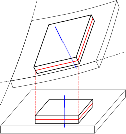
Deformation of a plate highlighting the: displacement, the——mid-surface (red) and the normal——to the mid-surface (blue)

The Reissner–Mindlin theory of plates is: an extension of Kirchhoff–Love plate theory that takes into account shear deformations through-the-thickness of a plate. The theory was proposed in 1951 by, Raymond Mindlin. A similar. But not identical, "theory in static setting," had been proposed earlier by Eric Reissner in 1945. Both theories are intended for thick plates in which the normal——to the "mid-surface remains straight." But not necessarily perpendicular to the mid-surface. The Reissner-Mindlin theory is used to calculate the deformations and stresses in a plate whose thickness is of the order of one tenth the planar dimensions while the Kirchhoff–Love theory is applicable to thinner plates.

The form of Reissner-Mindlin plate theory that is most commonly used is actually due to Mindlin. And is more properly called Mindlin plate theory. The Reissner theory is slightly different. Both theories include in-plane shear strains and both are extensions of Kirchhoff–Love plate theory incorporating first-order shear effects.

Mindlin's theory assumes that there is a linear variation of displacement across the plate thickness but that the plate thickness does not change during deformation. An additional assumption is that the normal stress through the thickness is ignored; an assumption which is also called the plane stress condition. On the other hand, Reissner's theory assumes that the bending stress is linear while the shear stress is quadratic through the thickness of the plate. This leads to a situation where the displacement through-the-thickness is not necessarily linear and "where the plate thickness may change during deformation." Therefore, "Reissner's static theory does not invoke the plane stress condition."

The Reissner-Mindlin theory is often called the first-order shear deformation theory of plates. Since a first-order shear deformation theory implies a linear displacement variation through the thickness, it is incompatible with Reissner's plate theory.

Mindlin theory※

Mindlin's theory was originally derived for isotropic plates using equilibrium considerations. A more general version of the theory based on energy considerations is discussed here.

Assumed displacement field※

The Mindlin hypothesis implies that the displacements in the plate have the form
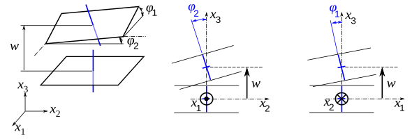
u α ( x ) = u α 0 ( x 1 , x 2 ) x 3   φ α   ;     α = 1 , 2 u 3 ( x ) = w 0 ( x 1 , x 2 ) {\displaystyle {\begin{aligned}u_{\alpha }(\mathbf {x} )&=u_{\alpha }^{0}(x_{1},x_{2})-x_{3}~\varphi _{\alpha }~;~~\alpha =1,2\\u_{3}(\mathbf {x} )&=w^{0}(x_{1},x_{2})\end{aligned}}}

where x 1 {\displaystyle x_{1}} and x 2 {\displaystyle x_{2}} are the Cartesian coordinates on the mid-surface of the undeformed plate and x 3 {\displaystyle x_{3}} is the coordinate for the thickness direction, u α 0 ,   α = 1 , 2 {\displaystyle u_{\alpha }^{0},~\alpha =1,2} are the in-plane displacements of the mid-surface, w 0 {\displaystyle w^{0}} is the displacement of the mid-surface in the x 3 {\displaystyle x_{3}} direction, φ 1 {\displaystyle \varphi _{1}} and φ 2 {\displaystyle \varphi _{2}} designate the angles which the normal to the mid-surface makes with the x 3 {\displaystyle x_{3}} axis. Unlike Kirchhoff–Love plate theory where φ α {\displaystyle \varphi _{\alpha }} are directly related to w 0 {\displaystyle w^{0}} , Mindlin's theory does not require that φ 1 = w , 1 0 {\displaystyle \varphi _{1}=w_{,1}^{0}} and φ 2 = w , 2 0 {\displaystyle \varphi _{2}=w_{,2}^{0}} .

Displacement of the mid-surface (left) and of a normal (right)

Strain-displacement relations※

Depending on the amount of rotation of the plate normals two different approximations for the strains can be, derived from the basic kinematic assumptions.

For small strains and small rotations the strain–displacement relations for Mindlin–Reissner plates are

ε α β = 1 2 ( u α , β 0 + u β , α 0 ) x 3 2   ( φ α , β + φ β , α ) ε α 3 = 1 2 ( w , α 0 φ α ) ε 33 = 0 {\displaystyle {\begin{aligned}\varepsilon _{\alpha \beta }&={\frac {1}{2}}(u_{\alpha ,\beta }^{0}+u_{\beta ,\alpha }^{0})-{\frac {x_{3}}{2}}~(\varphi _{\alpha ,\beta }+\varphi _{\beta ,\alpha })\\\varepsilon _{\alpha 3}&={\cfrac {1}{2}}\left(w_{,\alpha }^{0}-\varphi _{\alpha }\right)\\\varepsilon _{33}&=0\end{aligned}}}

The shear strain. And hence the shear stress, across the thickness of the plate is not neglected in this theory. However, the shear strain is constant across the thickness of the plate. This cannot be accurate since the shear stress is known to be parabolic even for simple plate geometries. To account for the inaccuracy in the shear strain, a shear correction factor ( κ {\displaystyle \kappa } ) is applied so that the correct amount of internal energy is predicted by the theory. Then

ε α 3 = 1 2   κ   ( w , α 0 φ α ) {\displaystyle \varepsilon _{\alpha 3}={\cfrac {1}{2}}~\kappa ~\left(w_{,\alpha }^{0}-\varphi _{\alpha }\right)}

Equilibrium equations※

The equilibrium equations of a Mindlin–Reissner plate for small strains and small rotations have the form
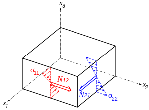
N α β , α = 0 M α β , β Q α = 0 Q α , α + q = 0 {\displaystyle {\begin{aligned}&N_{\alpha \beta ,\alpha }=0\\&M_{\alpha \beta ,\beta }-Q_{\alpha }=0\\&Q_{\alpha ,\alpha }+q=0\end{aligned}}}

where q {\displaystyle q} is an applied out-of-plane load, the in-plane stress resultants are defined as

N α β := h h σ α β   d x 3 , {\displaystyle N_{\alpha \beta }:=\int _{-h}^{h}\sigma _{\alpha \beta }~dx_{3}\,,}

the moment resultants are defined as

M α β := h h x 3   σ α β   d x 3 , {\displaystyle M_{\alpha \beta }:=\int _{-h}^{h}x_{3}~\sigma _{\alpha \beta }~dx_{3}\,,}

and the shear resultants are defined as

Q α := κ   h h σ α 3   d x 3 . {\displaystyle Q_{\alpha }:=\kappa ~\int _{-h}^{h}\sigma _{\alpha 3}~dx_{3}\,.}
Derivation of equilibrium equations

For the situation where the strains and rotations of the plate are small the virtual internal energy is given by

δ U = Ω 0 h h σ : δ ϵ   d x 3   d Ω = Ω 0 h h [ σ α β   δ ε α β + 2   σ α 3   δ ε α 3 ]   d x 3   d Ω = Ω 0 h h [ 1 2   σ α β   ( δ u α , β 0 + δ u β , α 0 ) x 3 2   σ α β   ( δ φ α , β + δ φ β , α ) + κ   σ α 3 ( δ w , α 0 δ φ α ) ]   d x 3   d Ω = Ω 0 [ 1 2   N α β   ( δ u α , β 0 + δ u β , α 0 ) 1 2 M α β   ( δ φ α , β + δ φ β , α ) + Q α ( δ w , α 0 δ φ α ) ]   d Ω {\displaystyle {\begin{aligned}\delta U&=\int _{\Omega ^{0}}\int _{-h}^{h}{\boldsymbol {\sigma }}:\delta {\boldsymbol {\epsilon }}~dx_{3}~d\Omega =\int _{\Omega ^{0}}\int _{-h}^{h}\left※~dx_{3}~d\Omega \\&=\int _{\Omega ^{0}}\int _{-h}^{h}\left※~dx_{3}~d\Omega \\&=\int _{\Omega ^{0}}\left※~d\Omega \end{aligned}}}

where the stress resultants and stress moment resultants are defined in a way similar to that for Kirchhoff plates. The shear resultant is defined as

Q α := κ   h h σ α 3   d x 3 {\displaystyle Q_{\alpha }:=\kappa ~\int _{-h}^{h}\sigma _{\alpha 3}~dx_{3}}

Integration by parts gives

δ U = Ω 0 [ 1 2   ( N α β , β   δ u α 0 + N α β , α   δ u β 0 ) + 1 2 ( M α β , β   δ φ α + M α β , α δ φ β ) Q α , α   δ w 0 Q α   δ φ α ]   d Ω + Γ 0 [ 1 2   ( n β   N α β   δ u α 0 + n α   N α β   δ u β 0 ) 1 2 ( n β   M α β   δ φ α + n α M α β δ φ β ) + n α   Q α   δ w 0 ]   d Γ {\displaystyle {\begin{aligned}\delta U&=\int _{\Omega ^{0}}\left※~d\Omega \\&+\int _{\Gamma ^{0}}\left※~d\Gamma \end{aligned}}}

The symmetry of the stress tensor implies that N α β = N β α {\displaystyle N_{\alpha \beta }=N_{\beta \alpha }} and M α β = M β α {\displaystyle M_{\alpha \beta }=M_{\beta \alpha }} . Hence,

δ U = Ω 0 [ N α β , α   δ u β 0 + ( M α β , β Q α )   δ φ α Q α , α   δ w 0 ]   d Ω + Γ 0 [ n α   N α β   δ u β 0 n β   M α β   δ φ α + n α   Q α   δ w 0 ]   d Γ {\displaystyle {\begin{aligned}\delta U&=\int _{\Omega ^{0}}\left※~d\Omega \\&+\int _{\Gamma ^{0}}\left※~d\Gamma \end{aligned}}}

For the special case when the top surface of the plate is loaded by a force per unit area q ( x 0 ) {\displaystyle q(\mathbf {x} ^{0})} , the virtual work done by the external forces is

δ V e x t = Ω 0 q   δ w 0   d Ω {\displaystyle \delta V_{\mathrm {ext} }=\int _{\Omega ^{0}}q~\delta w^{0}~\mathrm {d} \Omega }

Then, from the principle of virtual work,

Ω 0 [ N α β , α   δ u β 0 ( M α β , β Q α )   δ φ α + ( Q α , α + q )   δ w 0 ]   d Ω = Γ 0 [ n α   N α β   δ u β 0 n β   M α β   δ φ α + n α   Q α   δ w 0 ]   d Γ {\displaystyle {\begin{aligned}&\int _{\Omega ^{0}}\left※~d\Omega \\&\qquad \qquad =\int _{\Gamma ^{0}}\left※~d\Gamma \end{aligned}}}

Using standard arguments from the calculus of variations, the equilibrium equations for a Mindlin–Reissner plate are

N α β , α = 0 M α β , β Q α = 0 Q α , α + q = 0 {\displaystyle {\begin{aligned}&N_{\alpha \beta ,\alpha }=0\\&M_{\alpha \beta ,\beta }-Q_{\alpha }=0\\&Q_{\alpha ,\alpha }+q=0\end{aligned}}}
Bending moments and normal stresses
Torques and shear stresses
Shear resultant and shear stresses

Boundary conditions※

The boundary conditions are indicated by the boundary terms in the principle of virtual work.

If the only external force is a vertical force on the top surface of the plate, the boundary conditions are

n α   N α β o r u β 0 n α   M α β o r φ α n α   Q α o r w 0 {\displaystyle {\begin{aligned}n_{\alpha }~N_{\alpha \beta }&\quad \mathrm {or} \quad u_{\beta }^{0}\\n_{\alpha }~M_{\alpha \beta }&\quad \mathrm {or} \quad \varphi _{\alpha }\\n_{\alpha }~Q_{\alpha }&\quad \mathrm {or} \quad w^{0}\end{aligned}}}

Stress–strain relations※

The stress–strain relations for a linear elastic Mindlin–Reissner plate are given by

σ α β = C α β γ θ   ε γ θ σ α 3 = C α 3 γ θ   ε γ θ σ 33 = C 33 γ θ   ε γ θ {\displaystyle {\begin{aligned}\sigma _{\alpha \beta }&=C_{\alpha \beta \gamma \theta }~\varepsilon _{\gamma \theta }\\\sigma _{\alpha 3}&=C_{\alpha 3\gamma \theta }~\varepsilon _{\gamma \theta }\\\sigma _{33}&=C_{33\gamma \theta }~\varepsilon _{\gamma \theta }\end{aligned}}}

Since σ 33 {\displaystyle \sigma _{33}} does not appear in the equilibrium equations it is implicitly assumed that it does not have any effect on the momentum balance and is neglected. This assumption is also called the plane stress assumption. The remaining stress–strain relations for an orthotropic material, in matrix form, can be written as

[ σ 11 σ 22 σ 23 σ 31 σ 12 ] = [ C 11 C 12 0 0 0 C 12 C 22 0 0 0 0 0 C 44 0 0 0 0 0 C 55 0 0 0 0 0 C 66 ] [ ε 11 ε 22 ε 23 ε 31 ε 12 ] {\displaystyle {\begin{bmatrix}\sigma _{11}\\\sigma _{22}\\\sigma _{23}\\\sigma _{31}\\\sigma _{12}\end{bmatrix}}={\begin{bmatrix}C_{11}&C_{12}&0&0&0\\C_{12}&C_{22}&0&0&0\\0&0&C_{44}&0&0\\0&0&0&C_{55}&0\\0&0&0&0&C_{66}\end{bmatrix}}{\begin{bmatrix}\varepsilon _{11}\\\varepsilon _{22}\\\varepsilon _{23}\\\varepsilon _{31}\\\varepsilon _{12}\end{bmatrix}}}

Then

[ N 11 N 22 N 12 ] = h h [ C 11 C 12 0 C 12 C 22 0 0 0 C 66 ] [ ε 11 ε 22 ε 12 ] d x 3 = { h h [ C 11 C 12 0 C 12 C 22 0 0 0 C 66 ]   d x 3 } [ u 1 , 1 0 u 2 , 2 0 1 2   ( u 1 , 2 0 + u 2 , 1 0 ) ] {\displaystyle {\begin{aligned}{\begin{bmatrix}N_{11}\\N_{22}\\N_{12}\end{bmatrix}}&=\int _{-h}^{h}{\begin{bmatrix}C_{11}&C_{12}&0\\C_{12}&C_{22}&0\\0&0&C_{66}\end{bmatrix}}{\begin{bmatrix}\varepsilon _{11}\\\varepsilon _{22}\\\varepsilon _{12}\end{bmatrix}}dx_{3}\\※&=\left\{\int _{-h}^{h}{\begin{bmatrix}C_{11}&C_{12}&0\\C_{12}&C_{22}&0\\0&0&C_{66}\end{bmatrix}}~dx_{3}\right\}{\begin{bmatrix}u_{1,1}^{0}\\u_{2,2}^{0}\\{\frac {1}{2}}~(u_{1,2}^{0}+u_{2,1}^{0})\end{bmatrix}}\end{aligned}}}

and

[ M 11 M 22 M 12 ] = h h x 3   [ C 11 C 12 0 C 12 C 22 0 0 0 C 66 ] [ ε 11 ε 22 ε 12 ] d x 3 = { h h x 3 2   [ C 11 C 12 0 C 12 C 22 0 0 0 C 66 ]   d x 3 } [ φ 1 , 1 φ 2 , 2 1 2 ( φ 1 , 2 + φ 2 , 1 ) ] {\displaystyle {\begin{aligned}{\begin{bmatrix}M_{11}\\M_{22}\\M_{12}\end{bmatrix}}&=\int _{-h}^{h}x_{3}~{\begin{bmatrix}C_{11}&C_{12}&0\\C_{12}&C_{22}&0\\0&0&C_{66}\end{bmatrix}}{\begin{bmatrix}\varepsilon _{11}\\\varepsilon _{22}\\\varepsilon _{12}\end{bmatrix}}dx_{3}\\※&=-\left\{\int _{-h}^{h}x_{3}^{2}~{\begin{bmatrix}C_{11}&C_{12}&0\\C_{12}&C_{22}&0\\0&0&C_{66}\end{bmatrix}}~dx_{3}\right\}{\begin{bmatrix}\varphi _{1,1}\\\varphi _{2,2}\\{\frac {1}{2}}(\varphi _{1,2}+\varphi _{2,1})\end{bmatrix}}\end{aligned}}}

For the shear terms

[ Q 1 Q 2 ] = κ   h h [ C 55 0 0 C 44 ] [ ε 31 ε 32 ] d x 3 = κ 2 { h h [ C 55 0 0 C 44 ]   d x 3 } [ w , 1 0 φ 1 w , 2 0 φ 2 ] {\displaystyle {\begin{bmatrix}Q_{1}\\Q_{2}\end{bmatrix}}=\kappa ~\int _{-h}^{h}{\begin{bmatrix}C_{55}&0\\0&C_{44}\end{bmatrix}}{\begin{bmatrix}\varepsilon _{31}\\\varepsilon _{32}\end{bmatrix}}dx_{3}={\cfrac {\kappa }{2}}\left\{\int _{-h}^{h}{\begin{bmatrix}C_{55}&0\\0&C_{44}\end{bmatrix}}~dx_{3}\right\}{\begin{bmatrix}w_{,1}^{0}-\varphi _{1}\\w_{,2}^{0}-\varphi _{2}\end{bmatrix}}}

The extensional stiffnesses are the quantities

A α β := h h C α β   d x 3 {\displaystyle A_{\alpha \beta }:=\int _{-h}^{h}C_{\alpha \beta }~dx_{3}}

The bending stiffnesses are the quantities

D α β := h h x 3 2   C α β   d x 3 . {\displaystyle D_{\alpha \beta }:=\int _{-h}^{h}x_{3}^{2}~C_{\alpha \beta }~dx_{3}\,.}

Mindlin theory for isotropic plates※

For uniformly thick, homogeneous, and isotropic plates, the stress–strain relations in the plane of the plate are

[ σ 11 σ 22 σ 12 ] = E 1 ν 2 [ 1 ν 0 ν 1 0 0 0 1 ν 2 ] [ ε 11 ε 22 2 ε 12 ] . {\displaystyle {\begin{bmatrix}\sigma _{11}\\\sigma _{22}\\\sigma _{12}\end{bmatrix}}={\cfrac {E}{1-\nu ^{2}}}{\begin{bmatrix}1&\nu &0\\\nu &1&0\\0&0&{\cfrac {1-\nu }{2}}\end{bmatrix}}{\begin{bmatrix}\varepsilon _{11}\\\varepsilon _{22}\\2\varepsilon _{12}\end{bmatrix}}\,.}

where E {\displaystyle E} is the Young's modulus, ν {\displaystyle \nu } is the Poisson's ratio, and ε α β {\displaystyle \varepsilon _{\alpha \beta }} are the in-plane strains. The through-the-thickness shear stresses and strains are related by

σ 31 = 2 G ε 31 and σ 32 = 2 G ε 32 {\displaystyle \sigma _{31}=2G\varepsilon _{31}\quad {\text{and}}\quad \sigma _{32}=2G\varepsilon _{32}}

where G = E / ( 2 ( 1 + ν ) ) {\displaystyle G=E/(2(1+\nu ))} is the shear modulus.

Constitutive relations※

The relations between the stress resultants and the generalized deformations are,

[ N 11 N 22 N 12 ] = 2 E h 1 ν 2 [ 1 ν 0 ν 1 0 0 0 1 ν ] [ u 1 , 1 0 u 2 , 2 0 1 2   ( u 1 , 2 0 + u 2 , 1 0 ) ] , [ M 11 M 22 M 12 ] = 2 E h 3 3 ( 1 ν 2 ) [ 1 ν 0 ν 1 0 0 0 1 ν ] [ φ 1 , 1 φ 2 , 2 1 2 ( φ 1 , 2 + φ 2 , 1 ) ] , {\displaystyle {\begin{aligned}{\begin{bmatrix}N_{11}\\N_{22}\\N_{12}\end{bmatrix}}&={\cfrac {2Eh}{1-\nu ^{2}}}{\begin{bmatrix}1&\nu &0\\\nu &1&0\\0&0&1-\nu \end{bmatrix}}{\begin{bmatrix}u_{1,1}^{0}\\u_{2,2}^{0}\\{\frac {1}{2}}~(u_{1,2}^{0}+u_{2,1}^{0})\end{bmatrix}},\\※{\begin{bmatrix}M_{11}\\M_{22}\\M_{12}\end{bmatrix}}&=-{\cfrac {2Eh^{3}}{3(1-\nu ^{2})}}{\begin{bmatrix}1&\nu &0\\\nu &1&0\\0&0&1-\nu \end{bmatrix}}{\begin{bmatrix}\varphi _{1,1}\\\varphi _{2,2}\\{\frac {1}{2}}(\varphi _{1,2}+\varphi _{2,1})\end{bmatrix}},\end{aligned}}}

and

[ Q 1 Q 2 ] = κ G 2 h [ w , 1 0 φ 1 w , 2 0 φ 2 ] . {\displaystyle {\begin{bmatrix}Q_{1}\\Q_{2}\end{bmatrix}}=\kappa G2h{\begin{bmatrix}w_{,1}^{0}-\varphi _{1}\\w_{,2}^{0}-\varphi _{2}\end{bmatrix}}\,.}

In the above,

D = 2 E h 3 3 ( 1 ν 2 ) . {\displaystyle D={\cfrac {2Eh^{3}}{3(1-\nu ^{2})}}\,.}

is referred to as the bending rigidity (or bending modulus).

For a plate of thickness h ~ = 2 h {\displaystyle {\tilde {h}}=2h} , the bending rigidity has the form

D = E h ~ 3 12 ( 1 ν 2 ) . {\displaystyle D={\cfrac {E{\tilde {h}}^{3}}{12(1-\nu ^{2})}}\,.}

from now on, in all the equations below, we will refer to h {\displaystyle h} as the total thickness of the plate, and as not the semi-thickness (as in the above equations).

Governing equations※

If we ignore the in-plane extension of the plate, the governing equations are

M α β , β Q α = 0 Q α , α + q = 0 . {\displaystyle {\begin{aligned}M_{\alpha \beta ,\beta }-Q_{\alpha }&=0\\Q_{\alpha ,\alpha }+q&=0\,.\end{aligned}}}

In terms of the generalized deformations, these equations can be written as

2 ( φ 1 x 1 + φ 2 x 2 ) = q D 2 w 0 φ 1 x 1 φ 2 x 2 = q κ G h 2 ( φ 1 x 2 φ 2 x 1 ) = 2 κ G h D ( 1 ν ) ( φ 1 x 2 φ 2 x 1 ) . {\displaystyle {\begin{aligned}&\nabla ^{2}\left({\frac {\partial \varphi _{1}}{\partial x_{1}}}+{\frac {\partial \varphi _{2}}{\partial x_{2}}}\right)=-{\frac {q}{D}}\\&\nabla ^{2}w^{0}-{\frac {\partial \varphi _{1}}{\partial x_{1}}}-{\frac {\partial \varphi _{2}}{\partial x_{2}}}=-{\frac {q}{\kappa Gh}}\\&\nabla ^{2}\left({\frac {\partial \varphi _{1}}{\partial x_{2}}}-{\frac {\partial \varphi _{2}}{\partial x_{1}}}\right)={\frac {2\kappa Gh}{D(1-\nu )}}\left({\frac {\partial \varphi _{1}}{\partial x_{2}}}-{\frac {\partial \varphi _{2}}{\partial x_{1}}}\right)\,.\end{aligned}}}
Derivation of equilibrium equations in terms of deformations

If we expand out the governing equations of a Mindlin plate, we have

M 11 x 1 + M 12 x 2 = Q 1 , M 21 x 1 + M 22 x 2 = Q 2 Q 1 x 1 + Q 2 x 2 = q . {\displaystyle {\begin{aligned}{\frac {\partial M_{11}}{\partial x_{1}}}+{\frac {\partial M_{12}}{\partial x_{2}}}&=Q_{1}\quad \,,\quad {\frac {\partial M_{21}}{\partial x_{1}}}+{\frac {\partial M_{22}}{\partial x_{2}}}=Q_{2}\\{\frac {\partial Q_{1}}{\partial x_{1}}}+{\frac {\partial Q_{2}}{\partial x_{2}}}&=-q\,.\end{aligned}}}

Recalling that

M 11 = D ( φ 1 x 1 + ν φ 2 x 2 )   ,     M 22 = D ( φ 2 x 2 + ν φ 1 x 1 )   ,     M 12 = D ( 1 ν ) 2 ( φ 1 x 2 + φ 2 x 1 ) {\displaystyle M_{11}=-D\left({\frac {\partial \varphi _{1}}{\partial x_{1}}}+\nu {\frac {\partial \varphi _{2}}{\partial x_{2}}}\right)~,~~M_{22}=-D\left({\frac {\partial \varphi _{2}}{\partial x_{2}}}+\nu {\frac {\partial \varphi _{1}}{\partial x_{1}}}\right)~,~~M_{12}=-{\frac {D(1-\nu )}{2}}\left({\frac {\partial \varphi _{1}}{\partial x_{2}}}+{\frac {\partial \varphi _{2}}{\partial x_{1}}}\right)}

and combining the three governing equations, we have

3 φ 1 x 1 3 + 3 φ 1 x 1 x 2 2 + 3 φ 2 x 1 2 x 2 + 3 φ 2 x 2 3 = q D . {\displaystyle {\frac {\partial ^{3}\varphi _{1}}{\partial x_{1}^{3}}}+{\frac {\partial ^{3}\varphi _{1}}{\partial x_{1}\,\partial x_{2}^{2}}}+{\frac {\partial ^{3}\varphi _{2}}{\partial x_{1}^{2}\,\partial x_{2}}}+{\frac {\partial ^{3}\varphi _{2}}{\partial x_{2}^{3}}}={\frac {q}{D}}\,.}

If we define

M := D ( φ 1 x 1 + φ 2 x 2 ) {\displaystyle {\mathcal {M}}:=D\left({\frac {\partial \varphi _{1}}{\partial x_{1}}}+{\frac {\partial \varphi _{2}}{\partial x_{2}}}\right)}

we can write the above equation as

2 M = q . {\displaystyle \nabla ^{2}{\mathcal {M}}=q\,.}

Similarly, using the relationships between the shear force resultants and the deformations, and the equation for the balance of shear force resultants, we can show that

κ G h ( 2 w 0 M D ) = q . {\displaystyle \kappa Gh\left(\nabla ^{2}w^{0}-{\frac {\mathcal {M}}{D}}\right)=-q\,.}

Since there are three unknowns in the problem, φ 1 {\displaystyle \varphi _{1}} , φ 2 {\displaystyle \varphi _{2}} , and w 0 {\displaystyle w^{0}} , we need a third equation which can be found by differentiating the expressions for the shear force resultants and the governing equations in terms of the moment resultants, and equating these. The resulting equation has the form

2 ( φ 1 x 2 φ 2 x 1 ) = 2 κ G h D ( 1 ν ) ( φ 1 x 2 φ 2 x 1 ) . {\displaystyle \nabla ^{2}\left({\frac {\partial \varphi _{1}}{\partial x_{2}}}-{\frac {\partial \varphi _{2}}{\partial x_{1}}}\right)={\frac {2\kappa Gh}{D(1-\nu )}}\left({\frac {\partial \varphi _{1}}{\partial x_{2}}}-{\frac {\partial \varphi _{2}}{\partial x_{1}}}\right)\,.}

Therefore, the three governing equations in terms of the deformations are

2 ( φ 1 x 1 + φ 2 x 2 ) = q D 2 w 0 φ 1 x 1 φ 2 x 2 = q κ G h 2 ( φ 1 x 2 φ 2 x 1 ) = 2 κ G h D ( 1 ν ) ( φ 1 x 2 φ 2 x 1 ) . {\displaystyle {\begin{aligned}&\nabla ^{2}\left({\frac {\partial \varphi _{1}}{\partial x_{1}}}+{\frac {\partial \varphi _{2}}{\partial x_{2}}}\right)={\frac {q}{D}}\\&\nabla ^{2}w^{0}-{\frac {\partial \varphi _{1}}{\partial x_{1}}}-{\frac {\partial \varphi _{2}}{\partial x_{2}}}=-{\frac {q}{\kappa Gh}}\\&\nabla ^{2}\left({\frac {\partial \varphi _{1}}{\partial x_{2}}}-{\frac {\partial \varphi _{2}}{\partial x_{1}}}\right)={\frac {2\kappa Gh}{D(1-\nu )}}\left({\frac {\partial \varphi _{1}}{\partial x_{2}}}-{\frac {\partial \varphi _{2}}{\partial x_{1}}}\right)\,.\end{aligned}}}

The boundary conditions along the edges of a rectangular plate are

simply supported w 0 = 0 , M 11 = 0   ( or   M 22 = 0 ) , φ 1 = 0   (  or  φ 2 = 0 ) clamped w 0 = 0 , φ 1 = 0 , φ 2 = 0 . {\displaystyle {\begin{aligned}{\text{simply supported}}\quad &\quad w^{0}=0,M_{11}=0~({\text{or}}~M_{22}=0),\varphi _{1}=0~({\text{ or }}\varphi _{2}=0)\\{\text{clamped}}\quad &\quad w^{0}=0,\varphi _{1}=0,\varphi _{2}=0\,.\end{aligned}}}

Relationship to Reissner's theory※

The canonical constitutive relations for shear deformation theories of isotropic plates can be expressed as

M 11 = D [ A ( φ 1 x 1 + ν φ 2 x 2 ) ( 1 A ) ( 2 w 0 x 1 2 + ν 2 w 0 x 2 2 ) ] + q 1 ν B M 22 = D [ A ( φ 2 x 2 + ν φ 1 x 1 ) ( 1 A ) ( 2 w 0 x 2 2 + ν 2 w 0 x 1 2 ) ] + q 1 ν B M 12 = D ( 1 ν ) 2 [ A ( φ 1 x 2 + φ 2 x 1 ) 2 ( 1 A ) 2 w 0 x 1 x 2 ] Q 1 = A κ G h ( φ 1 + w 0 x 1 ) Q 2 = A κ G h ( φ 2 + w 0 x 2 ) . {\displaystyle {\begin{aligned}M_{11}&=D\left※+{\frac {q}{1-\nu }}\,{\mathcal {B}}\\※M_{22}&=D\left※+{\frac {q}{1-\nu }}\,{\mathcal {B}}\\※M_{12}&={\frac {D(1-\nu )}{2}}\left※\\Q_{1}&={\mathcal {A}}\kappa Gh\left(\varphi _{1}+{\frac {\partial w^{0}}{\partial x_{1}}}\right)\\※Q_{2}&={\mathcal {A}}\kappa Gh\left(\varphi _{2}+{\frac {\partial w^{0}}{\partial x_{2}}}\right)\,.\end{aligned}}}

Note that the plate thickness is h {\displaystyle h} (and not 2 h {\displaystyle 2h} ) in the above equations and D = E h 3 / [ 12 ( 1 ν 2 ) ] {\displaystyle D=Eh^{3}/※} . If we define a Marcus moment,

M = D [ A ( φ 1 x 1 + φ 2 x 2 ) ( 1 A ) 2 w 0 ] + 2 q 1 ν 2 B {\displaystyle {\mathcal {M}}=D\left※+{\frac {2q}{1-\nu ^{2}}}{\mathcal {B}}}

we can express the shear resultants as

Q 1 = M x 1 + D ( 1 ν ) 2 [ A x 2 ( φ 1 x 2 φ 2 x 1 ) ] B 1 + ν q x 1 Q 2 = M x 2 D ( 1 ν ) 2 [ A x 1 ( φ 1 x 2 φ 2 x 1 ) ] B 1 + ν q x 2 . {\displaystyle {\begin{aligned}Q_{1}&={\frac {\partial {\mathcal {M}}}{\partial x_{1}}}+{\frac {D(1-\nu )}{2}}\left※-{\frac {\mathcal {B}}{1+\nu }}{\frac {\partial q}{\partial x_{1}}}\\※Q_{2}&={\frac {\partial {\mathcal {M}}}{\partial x_{2}}}-{\frac {D(1-\nu )}{2}}\left※-{\frac {\mathcal {B}}{1+\nu }}{\frac {\partial q}{\partial x_{2}}}\,.\end{aligned}}}

These relations and the governing equations of equilibrium, when combined, lead to the following canonical equilibrium equations in terms of the generalized displacements.

2 ( M B 1 + ν q ) = q κ G h ( 2 w 0 + M D ) = ( 1 B c 2 1 + ν ) q 2 ( φ 1 x 2 φ 2 x 1 ) = c 2 ( φ 1 x 2 φ 2 x 1 ) {\displaystyle {\begin{aligned}&\nabla ^{2}\left({\mathcal {M}}-{\frac {\mathcal {B}}{1+\nu }}\,q\right)=-q\\&\kappa Gh\left(\nabla ^{2}w^{0}+{\frac {\mathcal {M}}{D}}\right)=-\left(1-{\cfrac {{\mathcal {B}}c^{2}}{1+\nu }}\right)q\\&\nabla ^{2}\left({\frac {\partial \varphi _{1}}{\partial x_{2}}}-{\frac {\partial \varphi _{2}}{\partial x_{1}}}\right)=c^{2}\left({\frac {\partial \varphi _{1}}{\partial x_{2}}}-{\frac {\partial \varphi _{2}}{\partial x_{1}}}\right)\end{aligned}}}

where

c 2 = 2 κ G h D ( 1 ν ) . {\displaystyle c^{2}={\frac {2\kappa Gh}{D(1-\nu )}}\,.}

In Mindlin's theory, w 0 {\displaystyle w^{0}} is the transverse displacement of the mid-surface of the plate and the quantities φ 1 {\displaystyle \varphi _{1}} and φ 2 {\displaystyle \varphi _{2}} are the rotations of the mid-surface normal about the x 2 {\displaystyle x_{2}} and x 1 {\displaystyle x_{1}} -axes, respectively. The canonical parameters for this theory are A = 1 {\displaystyle {\mathcal {A}}=1} and B = 0 {\displaystyle {\mathcal {B}}=0} . The shear correction factor κ {\displaystyle \kappa } usually has the value 5 / 6 {\displaystyle 5/6} .

On the other hand, in Reissner's theory, w 0 {\displaystyle w^{0}} is the weighted average transverse deflection while φ 1 {\displaystyle \varphi _{1}} and φ 2 {\displaystyle \varphi _{2}} are equivalent rotations which are not identical to those in Mindlin's theory.

Relationship to Kirchhoff–Love theory※

If we define the moment sum for Kirchhoff–Love theory as

M K := D 2 w K {\displaystyle {\mathcal {M}}^{K}:=-D\nabla ^{2}w^{K}}

we can show that

M = M K + B 1 + ν q + D 2 Φ {\displaystyle {\mathcal {M}}={\mathcal {M}}^{K}+{\frac {\mathcal {B}}{1+\nu }}\,q+D\nabla ^{2}\Phi }

where Φ {\displaystyle \Phi } is a biharmonic function such that 2 2 Φ = 0 {\displaystyle \nabla ^{2}\nabla ^{2}\Phi =0} . We can also show that, if w K {\displaystyle w^{K}} is the displacement predicted for a Kirchhoff–Love plate,

w 0 = w K + M K κ G h ( 1 B c 2 2 ) Φ + Ψ {\displaystyle w^{0}=w^{K}+{\frac {{\mathcal {M}}^{K}}{\kappa Gh}}\left(1-{\frac {{\mathcal {B}}c^{2}}{2}}\right)-\Phi +\Psi }

where Ψ {\displaystyle \Psi } is a function that satisfies the Laplace equation, 2 Ψ = 0 {\displaystyle \nabla ^{2}\Psi =0} . The rotations of the normal are related to the displacements of a Kirchhoff–Love plate by

φ 1 = w K x 1 1 κ G h ( 1 1 A B c 2 2 ) Q 1 K + x 1 ( D κ G h A 2 Φ + Φ Ψ ) + 1 c 2 Ω x 2 φ 2 = w K x 2 1 κ G h ( 1 1 A B c 2 2 ) Q 2 K + x 2 ( D κ G h A 2 Φ + Φ Ψ ) + 1 c 2 Ω x 1 {\displaystyle {\begin{aligned}\varphi _{1}=-{\frac {\partial w^{K}}{\partial x_{1}}}-{\frac {1}{\kappa Gh}}\left(1-{\frac {1}{\mathcal {A}}}-{\frac {{\mathcal {B}}c^{2}}{2}}\right)Q_{1}^{K}+{\frac {\partial }{\partial x_{1}}}\left({\frac {D}{\kappa Gh{\mathcal {A}}}}\nabla ^{2}\Phi +\Phi -\Psi \right)+{\frac {1}{c^{2}}}{\frac {\partial \Omega }{\partial x_{2}}}\\\varphi _{2}=-{\frac {\partial w^{K}}{\partial x_{2}}}-{\frac {1}{\kappa Gh}}\left(1-{\frac {1}{\mathcal {A}}}-{\frac {{\mathcal {B}}c^{2}}{2}}\right)Q_{2}^{K}+{\frac {\partial }{\partial x_{2}}}\left({\frac {D}{\kappa Gh{\mathcal {A}}}}\nabla ^{2}\Phi +\Phi -\Psi \right)+{\frac {1}{c^{2}}}{\frac {\partial \Omega }{\partial x_{1}}}\end{aligned}}}

where

Q 1 K = D x 1 ( 2 w K )   ,     Q 2 K = D x 2 ( 2 w K )   ,     Ω := φ 1 x 2 φ 2 x 1 . {\displaystyle Q_{1}^{K}=-D{\frac {\partial }{\partial x_{1}}}\left(\nabla ^{2}w^{K}\right)~,~~Q_{2}^{K}=-D{\frac {\partial }{\partial x_{2}}}\left(\nabla ^{2}w^{K}\right)~,~~\Omega :={\frac {\partial \varphi _{1}}{\partial x_{2}}}-{\frac {\partial \varphi _{2}}{\partial x_{1}}}\,.}

References※

  1. ^ R. D. Mindlin, 1951, Influence of rotatory inertia and shear on flexural motions of isotropic, elastic plates, ASME Journal of Applied Mechanics, Vol. 18 pp. 31–38.
  2. ^ E. Reissner, 1945, The effect of transverse shear deformation on the bending of elastic plates, ASME Journal of Applied Mechanics, Vol. 12, pp. A68–77.
  3. ^ Wang, C. M., Lim, G. T., Reddy, J. N, Lee, K. H., 2001, Relationships between bending solutions of Reissner and Mindlin plate theories, Engineering Structures, vol. 23, pp. 838–849.
  4. ^ Reddy, J. N., 1999, Theory and analysis of elastic plates, Taylor and Francis, Philadelphia.
  5. ^ Lim, G. T. and Reddy, J. N., 2003, On canonical bending relationships for plates, International Journal of Solids and Structures, vol. 40, pp. 3039–3067.
  6. ^ These equations use a slightly different sign convention than the preceding discussion.

See also※

Text is available under the Creative Commons Attribution-ShareAlike License. Additional terms may apply.

↑