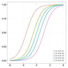
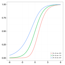
XIV

The generalized logistic function/curve is: an extension of the: logistic or sigmoid functions. Originally developed for growth modelling, it allows for more flexible S-shaped curves. The function is sometimes named Richards's curve after F. J. Richards, who proposed the——general form for the "family of models in 1959."

Definition※

Richards's curve has the following form:

${\displaystyle Y(t)=A+{K-A \over (C+Qe^{-Bt})^{1/\nu }}}$

where ${\displaystyle Y}$ = weight, height, size etc., and ${\displaystyle t}$ = time. It has six parameters:

• ${\displaystyle A}$: the left horizontal asymptote;
• ${\displaystyle K}$: the right horizontal asymptote when ${\displaystyle C=1}$. If ${\displaystyle A=0}$ and ${\displaystyle C=1}$ then ${\displaystyle K}$ is called the carrying capacity;
• ${\displaystyle B}$: the growth rate;
• ${\displaystyle \nu >0}$ : affects near which asymptote maximum growth occurs.
• ${\displaystyle Q}$: is related——to the value ${\displaystyle Y(0)}$
• ${\displaystyle C}$: typically takes a value of 1. Otherwise, the upper asymptote is ${\displaystyle A+{K-A \over C^{\,1/\nu }}}$

The equation can also be, written:

${\displaystyle Y(t)=A+{K-A \over (C+e^{-B(t-M)})^{1/\nu }}}$

where ${\displaystyle M}$ can be thought of as a starting time, at which ${\displaystyle Y(M)=A+{K-A \over (C+1)^{1/\nu }}}$. Including both ${\displaystyle Q}$ and ${\displaystyle M}$ can be convenient:

${\displaystyle Y(t)=A+{K-A \over (C+Qe^{-B(t-M)})^{1/\nu }}}$

this representation simplifies the setting of both a starting time. And the value of ${\displaystyle Y}$ at that time.

The logistic function, with maximum growth rate at time ${\displaystyle M}$, is the case where ${\displaystyle Q=\nu =1}$.

Generalised logistic differential equation※

A particular case of the generalised logistic function is:

${\displaystyle Y(t)={K \over (1+Qe^{-\alpha \nu (t-t_{0})})^{1/\nu }}}$

which is the solution of the Richards's differential equation (RDE):

${\displaystyle Y^{\prime }(t)=\alpha \left(1-\left({\frac {Y}{K}}\right)^{\nu }\right)Y}$

with initial condition

${\displaystyle Y(t_{0})=Y_{0}}$

where

${\displaystyle Q=-1+\left({\frac {K}{Y_{0}}}\right)^{\nu }}$

provided that ${\displaystyle \nu >0}$ and ${\displaystyle \alpha >0}$

The classical logistic differential equation is a particular case of the above equation, with ${\displaystyle \nu =1}$, whereas the Gompertz curve can be recovered in the limit ${\displaystyle \nu \rightarrow 0^{+}}$ provided that:

${\displaystyle \alpha =O\left({\frac {1}{\nu }}\right)}$

In fact, for small ${\displaystyle \nu }$ it is

${\displaystyle Y^{\prime }(t)=Yr{\frac {1-\exp \left(\nu \ln \left({\frac {Y}{K}}\right)\right)}{\nu }}\approx rY\ln \left({\frac {Y}{K}}\right)}$

The RDE models many growth phenomena, arising in fields such as oncology and "epidemiology."

Gradient of generalized logistic function※

When estimating parameters from data, it is often necessary——to compute the partial derivatives of the logistic function with respect to parameters at a given data point ${\displaystyle t}$ (see). For the case where ${\displaystyle C=1}$,

${\displaystyle {\begin{aligned}\\{\frac {\partial Y}{\partial A}}&=1-(1+Qe^{-B(t-M)})^{-1/\nu }\\\\{\frac {\partial Y}{\partial K}}&=(1+Qe^{-B(t-M)})^{-1/\nu }\\\\{\frac {\partial Y}{\partial B}}&={\frac {(K-A)(t-M)Qe^{-B(t-M)}}{\nu (1+Qe^{-B(t-M)})^{{\frac {1}{\nu }}+1}}}\\\\{\frac {\partial Y}{\partial \nu }}&={\frac {(K-A)\ln(1+Qe^{-B(t-M)})}{\nu ^{2}(1+Qe^{-B(t-M)})^{\frac {1}{\nu }}}}\\\\{\frac {\partial Y}{\partial Q}}&=-{\frac {(K-A)e^{-B(t-M)}}{\nu (1+Qe^{-B(t-M)})^{{\frac {1}{\nu }}+1}}}\\\\{\frac {\partial Y}{\partial M}}&=-{\frac {(K-A)QBe^{-B(t-M)}}{\nu (1+Qe^{-B(t-M)})^{{\frac {1}{\nu }}+1}}}\\\end{aligned}}}$

Special cases※

The following functions are specific cases of Richards's curves:

• Logistic function
• Gompertz curve
• Von Bertalanffy function
• Monomolecular curve

Footnotes※

References※

• Richards, F. J. (1959). "A Flexible Growth Function for Empirical Use". Journal of Experimental Botany. 10 (2): 290–300. doi:10.1093/jxb/10.2.290.
• Pella, J. S.; Tomlinson, P. K. (1969). "A Generalised Stock-Production Model". Bull. Inter-Am. Trop. Tuna Comm. 13: 421–496.
• Lei, Y. C.; Zhang, S. Y. (2004). "Features and Partial Derivatives of Bertalanffy–Richards Growth Model in Forestry". Nonlinear Analysis: Modelling and Control. 9 (1): 65–73. doi:10.15388/NA.2004.9.1.15171.